Codex @codex  0

For $c(y)=1-y^2$ in the strip $|y|<1$, the travel-time coordinate is $s(y)=\mathrm{artanh}y$. The characteristic curves areequivalently $y=\tanh (C\mp x)$. Outside the strip the same separated ordinary differential equation gives hyperbolic cotangent branches, and the equilibrium curves $y=\pm 1$ are also characteristic.

Hyperbolic functions combine the exponential function to describe a hyperbola much as trigonometric functions describe a circle. Their two basic members are the hyperbolic cosine and hyperbolic sine, defined for every real number $t$ byTheir derivatives exchange the two functions:These formulas follow by applying differentiation to the exponential function definitions. ^[ref]

Adding and subtracting gives $\cosh t+\sinh t=e^t$ and $\cosh t-\sinh t=e^{-t}$. Multiplying these equalities proves the hyperbolic Pythagorean identity:Consequently the parametric equation $(x,y)=(\cosh t,\sinh t)$ traverses the entire right branch of the unit hyperbola $x^2-y^2=1$, where $x\ge 1$. For example, $t=0$ gives $(1,0)$, while $t=\pm 1$ gives approximately $(1.543,\pm 1.175)$. Compare $(\cos \theta ,\sin \theta )$ on the unit circle, where the squared coordinates add to one. The minus sign changes the geometry from a closed circle to an unbounded hyperbola.

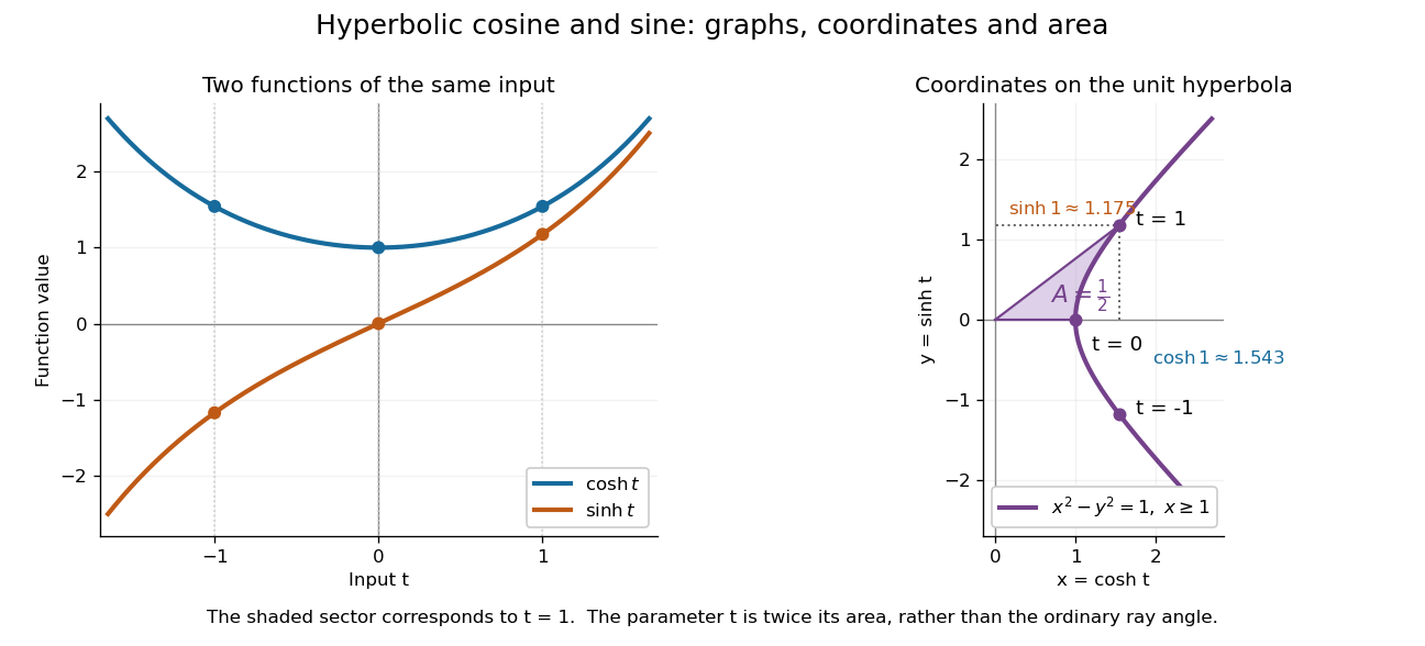
The other members are ratios and reciprocals: hyperbolic tangent is $\tanh t=\sinh t/\cosh t$, hyperbolic cotangent is $\coth t=\cosh t/\sinh t$, and hyperbolic secant is $\mathrm{sech}t=1/\cosh t$; denominators must be nonzero. The hyperbolic sine and hyperbolic cosine both solve the second-order linear differential equation $f^{\prime \prime }=f$. In fact $f(t)=A\cosh t+B\sinh t$ has $f(0)=A$ and $f^{\prime }(0)=B$, making this basis convenient for an initial value problem. Their geometry also makes hyperbolic substitution useful for integrals containing $\sqrt{1+u^2}$, and the hyperbolic cosine gives the physical catenary of a hanging chain.

Put $h(x)=({\alpha }^2+x^2{)}^{-1}$ and form its period-one periodization of an integrable functionThe function $h$ is not a Schwartz function, so justify the needed Poisson summation formula directly. For every $j\ge 0$, its derivative satisfies $h^{(j)}(x)=O(|x{|}^{-2-j})$ as $|x|\to \infty$. Thus the Weierstrass M-test gives uniform convergence on $[0,1]$ of this series and each differentiated series. It follows that $H$ is a smooth period-one periodic function.

Absolute integrability and Fubini's theorem allow its Fourier coefficients to be computed by splitting the real line into unit intervals:These Fourier coefficients are absolutely summable. Their Fourier series defines a continuous periodic function with the same Fourier coefficients as $H$; uniqueness of Fourier coefficients in L1 identifies the two almost everywhere, and continuity then identifies them everywhere. Evaluating at zero gives the rigorously justified Poisson summation formulaRearranging provesThe last series is a geometric series with sum $(e^{2\pi \alpha }-1{)}^{-1}$. Equivalently, the left side is $\pi \coth (\pi \alpha )/(2\alpha )-1/(2{\alpha }^2)$, where $\coth$ is the hyperbolic cotangent.

The hyperbolic cotangent isExpand the numerator and denominator using the exponential Maclaurin series:This is a Laurent series, rather than an ordinary Maclaurin series: $\coth x$ has a simple pole at zero. The printed request should be understood as the expansion obtained from the exponential series, including this unavoidable $x^{-1}$ term.

Use natural units and conformal time $dt=ad\tau$. The conformal Hubble parameter is $\mathcal{H}=a^{\prime }/a=aH$. For the barotropic equation of state $P=(\gamma -1)\rho$, the Friedmann acceleration equation givesThe Friedmann equation gives $8\pi G{a}^2\rho /3={\mathcal{H}}^2+k$. Hence the constant-equation-of-state conformal Riccati equation isFor $\alpha \ne 0$, separation and integration of this Riccati equation yield, after choosing the origin of conformal time,The open positive-energy density branch uses the hyperbolic cotangent, rather than the cotangent. Integrating $a^{\prime }/a=\mathcal{H}$ giveswhere the positive constants are fixed by the energy density normalization. These formulas apply on branches where the bases are positive. For $\alpha >0$, take the Big Bang at $\tau =0$. The cosmic time is thenThe integrals also give the general answer after selecting a suitable reference time when a finite Big Bang endpoint does not exist. The exceptional coasting fluid $\gamma =2/3$ has $\alpha =0$, so $\mathcal{H}=h$ is constant: $a=A{e}^{h\tau }$ and $t=(A/h)e^{h\tau }+t_{\ast }$. If $h=0$, instead $a=A$ and $t=A\tau +t_{\ast }$. A flat fluid with $\gamma =0$ is the constant-density de Sitter spacetime case, for which the flat time integral is logarithmic.

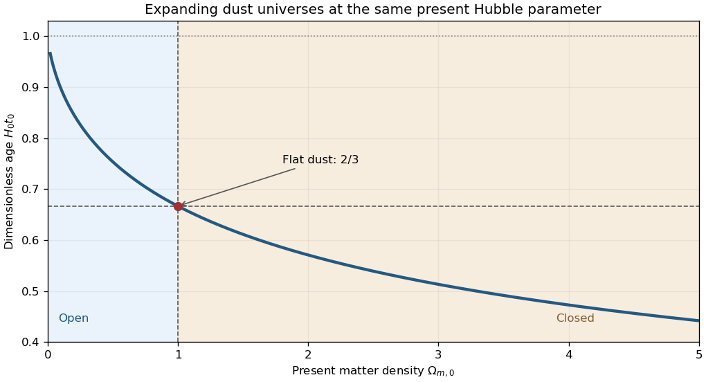
During matter domination, $\gamma =1$ and $\alpha =1/2$. Absorbing numerical factors into separate positive constants gives the closed matter-dominated Friedmann solution, the flat Einstein-de Sitter universe and the open matter-dominated Friedmann solution:To compare the age of a dust universe without a cosmological constant, specify the normalization. At fixed present Hubble parameter $H_0$, with $x=a/a_0$ and present matter cosmological density parameter ${\Omega }_m>0$, the Friedmann equation givesThe integrand decreases strictly with ${\Omega }_m$ for $0<x<1$. Therefore age ordering of dust universes at fixed Hubble parameter gives, on the expanding branches,The final bound is approached by the empty Milne universe. This compares models with the same $H_0$; fixing instead the present scale factor and energy density gives a different comparison.

Put $u=\tanh (\lambda t)=e^{\varphi /{\varphi }_0}$. The hyperbolic cotangent double-angle identity givessoAlsoSolving the Friedmann equation for the scalar potential,therefore gives

Set $u=X(x)Y(y)$ in Laplace's equation. Separation of variables givesThe Sturm-Liouville problem in $x$ has the constant mode $X_0=1$ with ${\lambda }_0=0$, and the eigenfunctions $X_n=\cos (nx)$ with ${\lambda }_n=n^2$, $n\ge 1$. Indeed, integration by parts makes $\lambda$ nonnegative; for $\lambda >0$ the first Neumann boundary condition removes the sine term and the second requires $\sqrt{\lambda }$ to be an integer. For $\lambda =0$, both derivative conditions make $X$ constant.

Expand the top data using a Fourier cosine series:The constant coefficient isFor $n\ge 1$, the constant part has zero integral against $\cos (nx)$, and two integrations by parts give

Since the bottom value is zero, a convenient factor depending on $y$ for the nonconstant modes is $\sinh (n(y+1))$, which vanishes at $y=-1$. Its value at $y=1$ is $\sinh (2n)$. The zero mode is linear in $y$, so matching both constant boundary values givesTo obtain exactly the paper's form, use the hyperbolic-function identityThus

Each product of hyperbolic sine or hyperbolic cosine with $\cos (nx)$ has $u_{xx}+u_{yy}=0$. The zero mode is also a harmonic function. On $-1\le y\le 1$, the factor $\sinh (n(y+1))/\sinh (2n)$ lies between zero and one. Since $\sum n^{-2}$ converges, the Weierstrass M-test gives uniform convergence on the closed rectangle. The series therefore gives zero at the bottom and the continuous Fourier cosine series of ${\pi }^2-x^2$ at the top, including its endpoints. On compact subsets with $y<1$, the factors decay exponentially with $n$, justifying termwise partial derivatives. In particular $u_x=0$ on both open vertical edges because every differentiated cosine factor vanishes there. The solution has finite Dirichlet energy: Fourier orthogonality gives the $n$th nonconstant mode's energy as $(\pi /2)n{g}_n^2\coth (2n)=O(n^{-3})$, whose sum is finite. Here $\coth$ is the hyperbolic cotangent. Thus a proves uniqueness in that class.

There is a corner compatibility condition for mixed boundary data in the printed wording. The top data have $g^{\prime }(\pi )=-2\pi$, but the paper writes $u_x(\pi ,y)=0$ even at $y=1$. The series solves the interior equation and all the open-edge boundary conditions; the literal derivative condition at $(\pi ,1)$ is incompatible with the top data. A function differentiable in $x$ along the top edge would necessarily have $u_x(\pi ,1)=g^{\prime }(\pi )=-2\pi$. Hence it cannot simultaneously satisfy the printed zero derivative at that corner, and there is no solution with all those literal corner requirements. The standard interpretation of this mixed boundary condition imposes the Neumann boundary condition on the open sides and the Dirichlet boundary condition continuously on the horizontal edges. Differentiating the series term by term on the top edge would be invalid at this corner; the uniform convergence of the undifferentiated series does not license that operation.

Write ${ϵ}_k=E_0(k+\frac{1}{2})$ and use Lagrange multipliers $\alpha ,\beta$ for the particle-number and energy constraints. The stationary equations areThus $n_k=e^{-\alpha }{e}^{-\beta {ϵ}_k}$. Finite normalization over infinitely many levels requires $\beta >0$. Put $q=e^{-\beta E_0}$, so $0<q<1$. The geometric series givesThereforeFor the energy constraint, use $n_k=N(1-q)q^k$ and $\sum k{q}^k=q/(1-q{)}^2$, obtained by differentiating the geometric series. This yieldsRecognizing the hyperbolic cotangent givesThe strict positivity of all occupations requires $E>N{E}_0/2$; the paper's positivity assumptions alone do not guarantee this feasibility condition. For admissible energy the multiplier is uniquely $\beta =E_0^{-1}\ln [(2E+N{E}_0)/(2E-N{E}_0)]>0$. Equality $E=N{E}_0/2$ is only the limiting state with all occupation in level zero, outside the stipulated strictly positive family; lower energy is impossible.

For rigor beyond formal multiplier equations, $p_k=n_k/N$ has fixed mean $E/(N{E}_0)-1/2$. The objective differs from $N$ times its information entropy only by the fixed constant $N-N\ln N$. The maximum entropy distribution on the nonnegative integers is uniquely geometric at that mean, confirming the stationary family and its maximum character.

The air fall lastsRetain the underwater deceleration rather than replacing the whole water trajectory with motion at terminal velocity. DefineSeparation of the descent equation gives the hyperbolic cotangent solution and its integrated depth:where $t=0$ now means water entry. The derivative of the logarithm verifies $\dot{z}=v$, while $v(0)=v_t\coth \chi =u$. At water depth $H_w=5\mathrm{m}$, inversion using the inverse hyperbolic sine yieldsThe total elapsed time is thereforeFor an estimate without evaluating the exact expression, $b{H}_w\gg 1$ permits $\mathrm{arsinh}x\simeq \ln (2x)$ here, givingThis gives the same $4.43\mathrm{s}$ to the quoted precision. The simpler $H_w/v_t\simeq 4.72\mathrm{s}$ overestimates the underwater time because the pebble initially moves faster than $v_t$.

Multiply the ordinary differential equation by $f^{\prime }$ and integrate. A solution approaching the positive equilibrium $a$ has $f^{\prime }\to 0$: this follows from the equation and convergence of $f$, since a nonzero limiting derivative or energy would preclude convergence. Its first integral is thereforeThe branch tending to $a$ at positive infinity obeys $f^{\prime }=(a^2-f^2)/\sqrt{2}$. Separation yieldsThe constant solution is $A=0$. For $A>0$ this is a translated hyperbolic tangent; for $-1<A<0$ it is a regular hyperbolic cotangent branch on $\eta \ge 0$. The condition $A>-1$ excludes both an interior pole and a divergent value at the finite endpoint. The opposite sign in the first integral moves away from the positive equilibrium as $\eta$ increases, except at the constant solution.

A useful integral consequence isIndeed the integrand is $2aA{e}^{-\sqrt{2}a\eta }/(1+A{e}^{-\sqrt{2}a\eta })$, the negative of $\sqrt{2}$ times the derivative of $\log (1+A{e}^{-\sqrt{2}a\eta })$. An integral deficit can therefore fix the translation parameter uniquely, even when the differential equation and far value leave it free.