The hypergeometric distribution counts marked objects in a uniformly chosen sample of fixed size from a finite population, using sampling without replacement. Let be the population size, let objects be marked, and sample distinct objects. If counts the marked objects selected, its probability mass function isThe bounds describe the support of a probability distribution and must be an integer; the mass is zero elsewhere. The denominator counts all size- subsets, while the numerator counts choices of marked and unmarked objects using binomial coefficients. This counting argument requires every size- sample to have the same probability.[ref]
https://web.mit.edu/14.380/www/handouts/hypergeometric.pdf. MIT 14.30, hypergeometric distribution handout, §§1–4
For a constructed example, a box contains ten labelled objects, four red and six blue. Select five without replacement. There are possible samples. The probabilities for areIn particular, . Five red objects are impossible because the box only contains four. The expected value is , and the variance is .
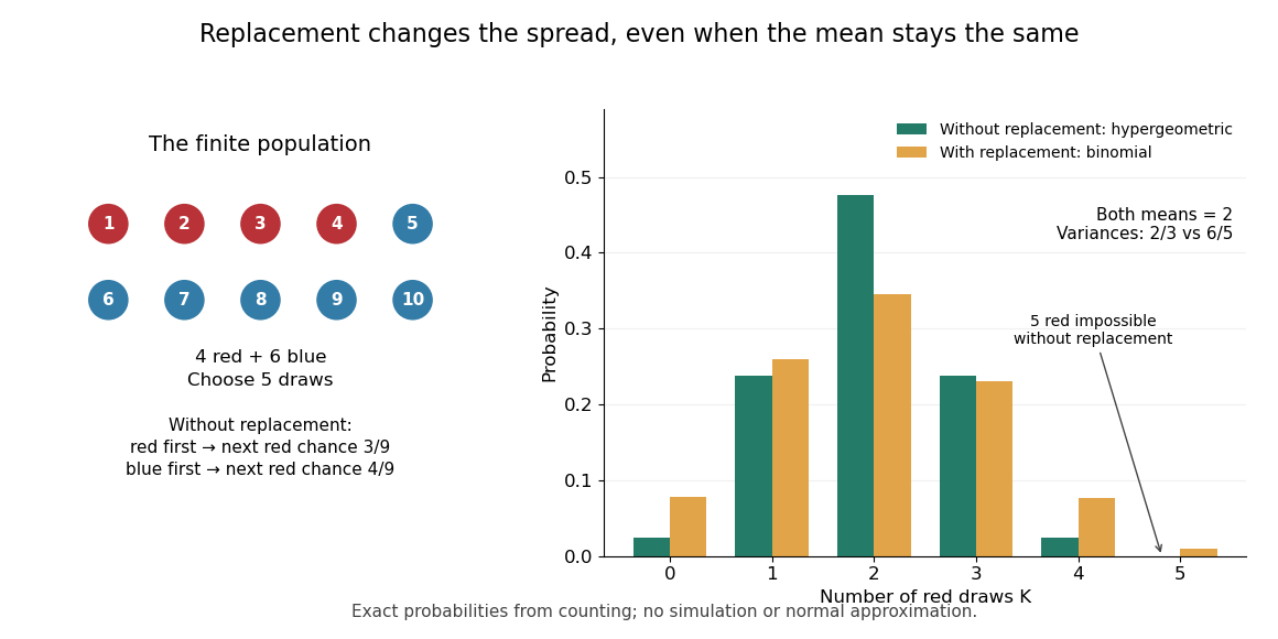
Five draws from four red and six blue objects: replacement preserves the mean but changes the spread
. Details. The count law also answers a detection question: what is the chance that five draws find at least one red object? By the complement rule of probability, it is , approximately . This can model inspecting five distinct objects from a known finite collection, with a mark indicating the property we want to detect. If repeated inspections can select the same object again, the replacement model instead gives . Equal expected values therefore do not imply equal chances of detecting a marked object.
The corresponding binomial distribution counts red draws when each selected object is put back before the next independent draw: . It has the same expected value , but variance , and it permits five red draws. Without replacement, a red first draw leaves red probability for the next draw; a blue first draw leaves . This statistical dependence pulls the total toward the fixed composition of the population, producing the finite population correction.
The useful modelling question is whether previously selected objects remain available. A fixed-size sample of distinct items calls for a hypergeometric distribution; fresh independent trials with constant success probability call for a binomial distribution. When the population grows with while stays fixed, the hypergeometric masses tend to the corresponding binomial distribution masses: removing finitely many objects has an increasingly small effect on the next draw's probability.
For uniform sampling without replacement from a population of objects, the finite population correction accounts for the reduced spread caused by drawing distinct objects. For the marked-object count in a hypergeometric distribution, put . ThenRelative to the corresponding binomial distribution, the variance is multiplied by and the standard deviation by . The square-root convention for the correction is used in Philip Stark's discussion of sample sums.[ref]
https://www.stat.berkeley.edu/~stark/SticiGui/Text/standardError.htm. Stark, SticiGui, Standard Error: sample sums without replacement
The factor has a direct interpretation. For , replacement makes no difference and . For , the entire population is observed and the marked count is exactly , so . In the ten-object, five-draw example, and . The exceptional population size is deterministic and should be handled directly rather than inserting it into a zero denominator.
A short explanation uses an indicator random variable for a marked object at draw . Each has expected value and variance . For distinct draw positions ,Since , the variance of a sum includes individual terms and ordered covariance terms, giving the displayed correction. Linearity of expectation still gives despite this dependence.
For arbitrary fixed real population values, use for population size and for sample size. Write the finite population mean , the finite population variance and . Under simple random sampling without replacement, the sample mean satisfiesThus is the variance factor relative to , while is the exact variance ratio to independent uniform sampling with replacement, whose sample mean has variance . The standard error uses the square root of the corresponding factor. These formulas agree because ; the denominator convention must be specified. The sample mean under simple random sampling gives a derivation and an exact six-value example.
Suppose a finite population is split into categories with fixed sizes summing to . A uniform size- sample drawn by sampling without replacement has category counts with the displayed joint probability mass function, for integers summing to . It extends the two-category hypergeometric distribution; replacing the sampled objects instead gives a multinomial distribution.
For a box with category sizes and a sample of four distinct objects, the count pattern has probabilityPut . When , its covariance matrix is the corresponding multinomial distribution covariance matrix multiplied by the squared finite population correction:This connects the fixed-total dependence between categories with the further reduction from sampling without replacement. X. G. Duan gives a symmetry-based explanation of this shared covariance structure.[ref]
https://arxiv.org/abs/2101.00548. Duan, Better understanding of the multivariate hypergeometric distribution, 2021 preprint
Articles by others on the same topic


The Hypergeometric distribution is a probability distribution that describes the likelihood of a certain number of successes in a sequence of draws from a finite population without replacement. It is particularly useful in scenarios where you are interested in sampling a small number of items from a larger group without putting them back into the group after each draw. ### Parameters of the Hypergeometric Distribution The Hypergeometric distribution is defined by the following parameters: 1. **N**: The population size (the total number of items).