A multinomial distribution describes category counts from independent trials, each choosing exactly one of categories with the same probabilities . Require to be an integer, , and . If counts the trials in category , then andThe are integers, and the mass is zero for other count patterns. A category with has count zero almost surely, with in this formula. For a specified ordered trial sequence, independence gives the product of numbers ; the multinomial coefficient counts the different sequences with that same count pattern.
For four trials with category probabilities , the count pattern can occur in orders, each of probability . Thus its total probability is . This is a constructed independent-trial example, distinct from drawing four objects without replacement from a ten-object population of composition , where the multivariate hypergeometric distribution gives .
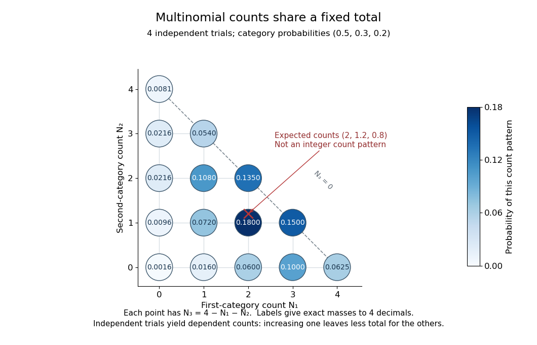
Three category counts from four independent trials: every point fixes the third count through the total
. Details. The diagram shows all fifteen possible count patterns. Coordinates determine ; the triangle is a constraint on integer counts, not a continuous probability density. The mode is , where the probability mass function is largest, but the expected values are not a possible count pattern.
Each single count has a binomial distribution, because recording category versus all other categories reduces every trial to a Bernoulli trial. Consequently,These statements about the joint count model are summarized in Aditya Guntuboyina's lecture notes.[ref]
https://stat238.berkeley.edu/spring-2026/lecturetwelve238spring2026/. Guntuboyina, Berkeley STAT 238, lecture 12: multinomial distribution
Independent trials do not make the resulting counts independent random variables. Within one trial the indicator random variables for two distinct categories cannot both equal one, so their product is zero and their covariance is . Summing over independent trials gives . In the four-trial example, the variances are and the pairwise covariances are . Knowing that all four trials were in the first category fixes the other two counts at zero.
The attraction is that one formula describes any fixed-total list of category counts while preserving the constraint that they add up to . It underlies multinomial likelihood calculations and uniform balls-in-bins allocation. The multinomial aggregation rule lets us merge categories without leaving this family of probability distributions. Allowing independent category counts with an unfixed total instead leads to a different model, related through Poisson-multinomial conditioning.
If has a multinomial distribution with trials, group its categories into disjoint nonempty sets covering all categories. The grouped counts in the displayed equation have the multinomial distributionEach original trial belongs to exactly one group, its group probability is the sum of its category probabilities, and grouping preserves independence between trials. This gives the rule without summing the original probability mass function over every possible internal count pattern.
For the four-trial example with probabilities , merge the last two categories. Their total has the binomial distribution , so and . The same variance follows from the variance of a sum:Ignoring the negative covariance would give , although the two counts share a fixed total. Multinomial aggregation lets the resolution of category labels change while retaining a consistent model for the counts.
For cell means with , the independent Poisson distribution likelihood and the multinomial distribution likelihood with probabilities differ by a parameter-independent factor. Thus a maximum-likelihood estimator for the unrestricted Poisson model whose fitted total is is also an estimator for the constrained multinomial model. Equality of named parameter estimates presumes identifiability and uniqueness; without these, the conclusion concerns the sets of maximizers. A free intercept in a log-linear Poisson model enforces the fitted-total equation.
Counts of several categories before a fixed number of stopping-category outcomes have a negative multinomial distribution. For one stopping outcome of probability , the two-count mass function is . Its probability generating function is and its means are and .
For independent one-stop negative multinomial distribution observations, the natural estimates are and . Their sum is with strictly concave , so Jensen's inequality makes its expectation strictly below . Conditional category proportions split this bias between both estimates. With zero observed counts of a category, that estimate lies at zero; in a parameter space requiring strict positivity the likelihood supremum is not attained.
The vector of category counts is the sum of independent categorical indicator vectors. Their means are and covariance is , so the multivariate central limit theorem gives the displayed limit. At uniform probabilities on categories, Pearson-standardized deviations have covariance equal to the orthogonal projection onto the -dimensional subspace of zero-sum vectors. Their squared norm has an asymptotic chi-squared distribution with degrees of freedom.
Place labelled balls independently into labelled bins, each with probability . The vector of bin counts has a multinomial distribution, and each count separately has the binomial distribution . Distinct bin counts have covariance , so they are dependent for and . Counts of bins of a specified size are sums of indicator variables; their expectations follow from the linearity of expectation, without any independence between bins.
In repeated uniform balls-in-bins allocation, remove each ball that is alone in its bin and independently reallocate all remaining balls in the next round. If balls remain, the conditional expectation of the next count is for , and zero for . The surviving-ball indicator random variables need not be independent. For two balls and two bins, both remain with probability after rounds, so .
For balls in uniformly and independently chosen boxes, put . The empty-box indicators in uniform allocation have negative pairwise covariance, so . Chebyshev's inequality givesSince , this proves the displayed convergence in probability. The centring and the negative covariance are essential to this short proof; an expectation limit alone would not establish concentration.
Place balls independently and uniformly into boxes. If indicates that box is empty, then , , and, for ,Indeed all balls avoid one specified box with probability and two specified boxes with probability . The indicator random variable identities give the expectations, variances, and covariance. Finally proves strict negativity. Thus the number of empty boxes has and by the variance of a sum.
In a uniform balls-in-bins allocation with and , a fixed bin count has convergence in distribution to a Poisson distribution variable of mean by the Poisson limit theorem. If counts bins containing exactly balls, symmetry and the linearity of expectation give for each fixed . In particular the expected empty fraction tends to , and the expected fraction with at least two balls tends to . These are statements about expectations; convergence of the random fractions requires an additional argument.
For category counts with fixed total and probabilities , the multinomial likelihood isIts maximum-likelihood fitted probabilities are .
For counts with a multinomial distribution, this is twice the log likelihood ratio of the saturated cell-probability estimate to fixed probabilities . Zero-count terms have limiting value zero. Simulation under the specified probabilities gives a direct reference distribution when asymptotic approximations are unsuitable.
A categorical distribution describes one trial with one of labelled outcomes and probabilities summing to one. The labels need not be numbers or have an order. It is the single-trial building block of the multinomial distribution: independent draws with the same categorical distribution produce multinomial category counts.
For a trial choosing labels with probabilities , the category-indicator random vector is , , or . Its expected value is ; its components are dependent because exactly one is one. A numerical encoding of is a separate modelling choice: the category labels themselves do not define an arithmetic mean.
Articles by others on the same topic


The multinomial distribution is a generalization of the binomial distribution. It describes the probabilities of obtaining a distribution of counts across more than two categories. While the binomial distribution is applicable when there are two possible outcomes (success or failure), the multinomial distribution is used when there are multiple outcomes.