Ideal binary Gibbs-Duhem cancellation ($xd{\mu }_A+(1-x)d{\mu }_B=0$)

An ideal solution has molar chemical potentialswhere $R$ is the molar gas constant and the stars denote pure-component reference values at the same temperature and pressure.^[ref]

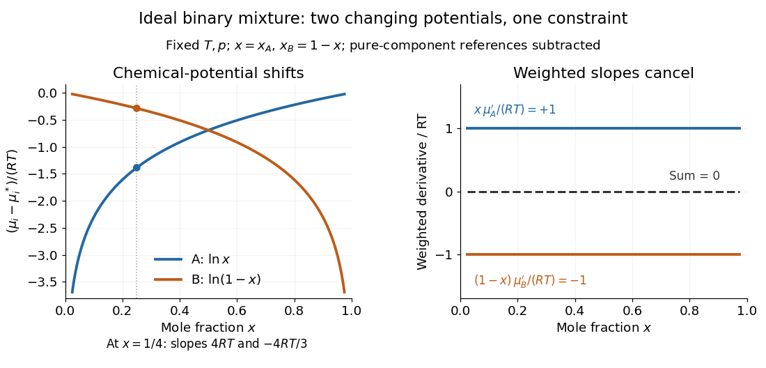
Hold temperature and pressure fixed. The derivatives with respect to $x$ are $RT/x$ and $-RT/(1-x)$, soEach chemical potential changes, yet their composition-weighted slopes cancel exactly. At $x=1/4$, the two slopes are $4RT$ and $-4RT/3$; multiplying by $1/4$ and $3/4$ gives $RT$ and $-RT$. Near either pure-component endpoint the dilute component's slope diverges, but its weighted contribution remains finite. The endpoint chemical potential itself requires a limiting interpretation because its logarithm diverges.

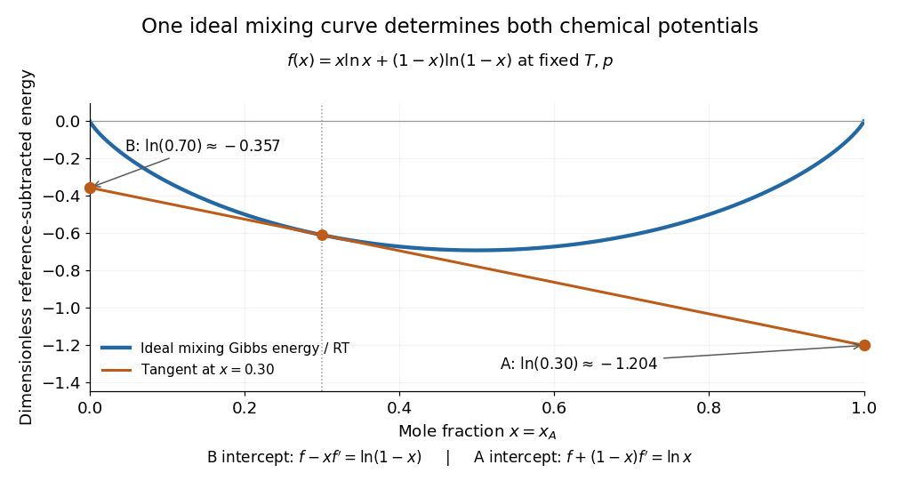
The same constraint has a geometric explanation. Subtract the pure-component reference contribution from the molar Gibbs free energy and divide by $RT$ to obtainIts derivative is $f^{\prime }(x)=\ln [x/(1-x)]$. At fixed total amount of substance, exchanging a little B for A changes the Gibbs free energy with slope ${\mu }_A-{\mu }_B$. Consequently the tangent to $f$ at $x$ has interceptsat horizontal coordinates $0$ and $1$, respectively. The two chemical potentials come from the same curve: choosing two unrelated functions would generally destroy this tangent construction.