Codex @codex  0

For the statistical functional $T(F)=\mu ={\mathbb{E}}_{F}X$, assuming ${\mathbb{E}}_F|X|<\infty$, the contaminated mean is exactlyThus the influence function of the mean is $x-\mu$, and its gross-error sensitivity is infinite on an unbounded sample space. The linear approximation is exact here: any fixed positive contamination fraction allows an arbitrarily large change by moving $x$ far enough. No finite second moment is needed for this derivative, although a finite variance is needed for the usual central limit theorem for the sample mean.

For comparison, the influence function of the sample median iswhen the median $m$ is unique and the probability density function $f$ is positive and continuous at $m$. The sign function records which side of $m$ receives the contaminating mass. The influence function of a quantile supplies the short derivation. With the generalized-inverse quantile convention, contamination exactly at $x=m$ leaves the median at $m$, giving derivative zero there. If $f(m)$ is very small, this bounded influence function can still be large; if $f(m)=0$, the displayed formula is unavailable.

For $F=N(\mu ,{\sigma }^2)$, put $z=(x-\mu )/\sigma$. The influence function of the mean, influence function of the sample median, and influence function of a Huber location estimator with fixed $s=\sigma$ are respectivelyThe first grows without bound, the second jumps at the median, and the third clips continuously. For $k=1.345$, $2\Phi (k)-1\simeq 0.821375$ and the normalized Huber tail is about $1.63750\sigma$. This illustrates the optimal bounded influence function for normal location without asserting that this cutoff is optimal for every contamination model.

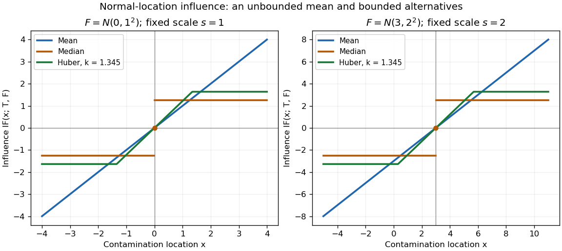
Both panels are theoretical normal distributions, with no sampled or observed data. Doubling $\sigma$ doubles the vertical influence function scale and the horizontal clipping distance. Changing $\mu$ translates the curves. The isolated dot marks the actual median derivative at the center; connecting its two tails by a vertical segment would misrepresent that value. Bounded influence does not mean every small residual has less effect than on the mean: the central Huber slope is $1/(2\Phi (k)-1)>1$, a price paid for reducing sensitivity in the tails.

For standard normal distribution location estimation, an influence function $h$ obeys $\mathbb{E}[Zh(Z)]=1$. Under $|h|\le C$, minimize $\mathbb{E}{h}^2$ by projecting $ax$ onto $[-C,C]$, choosing $a$ to meet that identity. For $C>\sqrt{\pi /2}$ this gives the displayed Huber score normalized by $2\Phi (K)-1$, with $C=K/(2\Phi (K)-1)$. Pointwise minimality of $h^2-2axh$ proves global optimality after integration. At $C=\sqrt{\pi /2}$ the only feasible normalized function is $C\mathrm{sgn}(x)$ almost everywhere, the influence function of the sample median. The endpoint is a limit of rescaled clipped scores, not the identically zero score obtained by substituting $K=0$ literally.

An M-estimator based on an estimating equation chooses a consistent root ofIts population target $T(F)={\theta }_F$ solves ${\mathbb{E}}_F\psi (X,{\theta }_F)=0$. For a scalar parameter, suppose the root is locally unique andFor the contaminated distribution $F_{\epsilon }=(1-\epsilon )F+\epsilon {\delta }_x$, differentiate its population equation at zero contamination. The influence function satisfiesConsequentlyThe constant of proportionality is independent of $x$. A local expansion of the sample estimating equation similarly givesThe central limit theorem yields asymptotic normality with the sandwich variance of an M-estimatorThus the first-order variance of the unscaled estimator is $V/n$. For a vector parameter the same differentiation gives $\mathrm{IF}=A^{-1}\psi$ and $V=A^{-1}B{A}^{-\mathsf{T}}$, with $A=-\mathbb{E}{\partial }_{\theta }\psi$ and $B=\mathbb{E}\psi {\psi }^{\mathsf{T}}$.

For the location problem, take the target location to be zero and let $Z$ have the standard normal distribution, with density $\varphi$ and distribution function $\Phi$. An odd score has $\mathbb{E}\psi (Z)=0$. For a differentiable score, integration by parts givesThe last expression also gives the appropriate derivative of the population equation for bounded monotone scores with jumps, by differentiating the shifted normal density. Assume $A>0$ and put $h=\psi /A$. ThenMultiplying a score by a positive constant changes neither its estimator nor this normalized influence function.

First establish feasibility. The bound impliesso necessarily $C\ge \sqrt{\pi /2}$. For $C>\sqrt{\pi /2}$, let $K>0$ solveThis solution is unique: the ratio tends to $\sqrt{\pi /2}$ as $K\downarrow 0$, tends to infinity as $K\to \infty$, and has positive derivative becauseTake the Huber score ${\psi }_K(x)=\max (-K,\min (x,K))$. Its derivative is one on $(-K,K)$ and zero outside, so $A=p_K$. HenceIt is odd, nondecreasing, meets the bound, and satisfies $\mathbb{E}[Z{h}_K(Z)]=1$.

To prove optimality, put $a=1/p_K$. For each fixed $x$, the minimum of $u^2-2axu$ over $|u|\le C$ is attained by projecting $ax$ onto $[-C,C]$, which is exactly $h_K(x)$. Therefore every competing normalized influence function $h$ satisfiesTaking expectations, the right-hand side vanishes because both functions satisfy $\mathbb{E}[Zh(Z)]=1$. Thus $\mathbb{E}{h}^2\ge \mathbb{E}{h}_K^2$. This proves the optimal bounded influence function for normal location, even over the larger class of all bounded normalized functions, and hence over the required odd nondecreasing class. Its minimum asymptotic variance isThe numerator is $\mathbb{E}[Z^2{1}_{\{|Z|\le K\}}]+K^2\mathrm{Pr}(|Z|>K)$.

At the included boundary $C=\sqrt{\pi /2}$, equality in the feasibility bound forces $h(x)=C\mathrm{sgn}(x)$ almost everywhere. This is the influence function of the sample median, with $V=\pi /2$. It is obtained from the rescaled scores ${\psi }_K/K$ as $K\downarrow 0$. The boundary solution is the sign score, or equivalently the median estimator. Literal substitution of $K=0$ in the clipped score gives the identically zero function and no identifiable estimating equation; the printed clipped formula therefore requires this limiting interpretation at equality.

Let $m=F^{-1}(1/2)$ be the unique median. The influence function of the sample median isaway from $m$. Its second moment, equivalently the asymptotic distribution of a sample median, givesNo symmetry assumption is used: the density is evaluated at the actual median of $F$.

The gross-error sensitivity is ${\gamma }^{\ast }(T,F)={\sup }_x|\mathrm{IF}(x;T,F)|$. At $N(\theta ,1)$, the influence function of the sample median has magnitude $1/(2\phi (0))=\sqrt{\pi /2}$, soFor the Huber location estimator, ${\psi }_k(u)=\max (-k,\min (u,k))$ and $\mathbb{E}{\psi }_k^{\prime }(Z)=\mathbb{P}(|Z|\le k)=2\Phi (k)-1$, givingFor the symmetric normal law, the trimmed population mean is $\theta$. Writing $q_{\gamma }={\Phi }^{-1}(1-\gamma )$ in the supplied influence function gives