Codex @codex  0

Here is an original reproducible finite set with 40 points and 512 coordinates. Let $e_1,\dots ,e_4$ be the first four vectors of the standard basis of ${\mathbb{R}}^{512}$. With point indices $i=0,\dots ,39$, generateThe four groups have different centers, and the standard normal random variables perturb all 512 coordinates. Generate the coordinates in row order using NumPy's PCG64 pseudorandom number generator with seed 20261013. Then keep this finite set fixed. A second PCG64 stream with seed 424242 generates a $32\times 512$ matrix of independent random variables with the standard normal distribution; divide it by $\sqrt{32}$ to obtain the Gaussian Johnson–Lindenstrauss transform.

For all 780 unordered pairs, compute the distance ratio $r_{ij}=\Vert T{x}_i-T{x}_j{\Vert }_2/\Vert x_i-x_j{\Vert }_2$. In this draw, its minimum is approximately $0.733010$ and its maximum $1.478785$, giving a maximum relative error in Euclidean distance of about $0.478785$. The squared-distance ratios $r_{ij}^2$ instead range from approximately $0.537304$ to $2.186806$: their maximum relative error is about $1.186806$. Thus this particular draw fails a 20% distance tolerance. The Johnson–Lindenstrauss lemma does not assert that every draw into 32 dimensions must succeed.

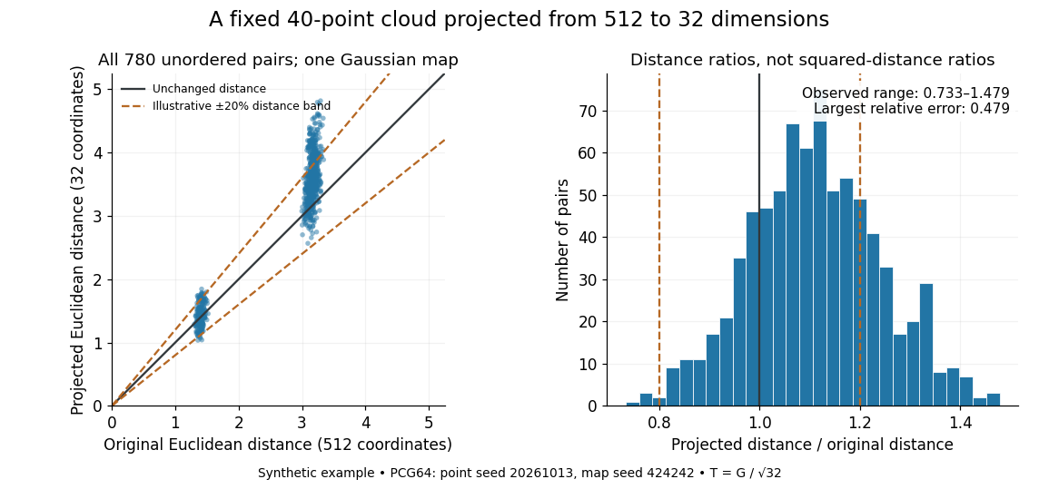
The two bands of original Euclidean distances distinguish pairs within a group from pairs between groups. Their spread after the linear map shows why checking an average distance is insufficient: the Johnson–Lindenstrauss lemma controls every pair. The dashed 20% distance band is an illustrative tolerance, not a confidence interval or a squared-distance band. The affine hull of 40 points has dimension at most 39; 512 is the ambient coordinate count, and no full-dimensionality assumption is required. For this draw the bi-Lipschitz distortion is approximately $1.478785/0.733010=2.017414$.

Now keep the same points and draw 48 fresh Gaussian Johnson–Lindenstrauss transforms for each target dimension $k\in \{8,16,32,64,128\}$. NumPy's SeedSequence(314159).spawn(240) supplies distinct PCG64 streams, ordered first by target dimension, then by draw. Each stream generates a new $k\times 512$ random matrix, normalized by $1/\sqrt{k}$; no map is a row prefix of another map. Each plotted value is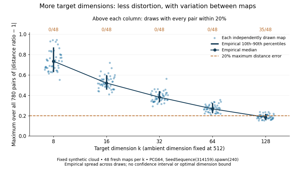

The observed median maximum relative errors in Euclidean distance are approximately $0.735$, $0.520$, $0.381$, $0.267$, and $0.184$, respectively. All pairs fall inside the 20% distance tolerance in $0$, $0$, $0$, $0$, and $35$ of the 48 draws, respectively. These are computations on one synthetic finite set, rather than optimal dimension bounds or measured physical data. The displayed quantiles describe the sampled maps; they do not certify a success probability for other sets. Even at 128 dimensions, 13 of the sampled maps fail this tolerance.

The practical benefit is that each point acquires fewer coordinates while its pairwise Euclidean distances can remain useful. The choice of target dimension balances compression, accuracy, and failure probability. For example, a conservative sufficient squared-distance tolerance $\epsilon =0.2$ with $n=40$ and $\delta =0.05$ gives $k\ge 1195$ by the explicit bound above. Here that exceeds the ambient dimension, so the identity map is better for a certified guarantee. The much smaller dimensions in the plots illustrate observed behavior without claiming that this sufficient bound is sharp.

For $0<\epsilon <1$ and any $n$ points in a Hilbert space, there is a linear map into Euclidean dimension $O({\epsilon }^{-2}\log n)$ that multiplies every pairwise distance by a factor between $1-\epsilon$ and $1+\epsilon$.

The striking feature is that the target dimension depends on the number of points and the allowed error, independently of the ambient dimension. Fix a finite set $S=\{x_1,\dots ,x_n\}\subset {\mathbb{R}}^D$, with $n\ge 2$, and $0<\epsilon <1$. An equivalent sufficient statement uses squared Euclidean distances: a linear map $T:{\mathbb{R}}^D\to {\mathbb{R}}^k$ exists, with $k=O({\epsilon }^{-2}\log n)$, such thatThe finite-set theorem cited here supplies an explicit sufficient target dimension for this squared-distance formulation. ^[ref]

Taking square roots gives distance factors $\sqrt{1-\epsilon }$ and $\sqrt{1+\epsilon }$, which lie inside $[1-\epsilon ,1+\epsilon ]$. Conversely, bounds $1\pm \epsilon$ on distances only give squared-distance bounds $(1\pm \epsilon {)}^2$; the same numerical tolerance should not be silently used for both. Under the squared-distance bounds, the bi-Lipschitz distortion is at most $\sqrt{(1+\epsilon )/(1-\epsilon )}$.

The Johnson–Lindenstrauss lemma preserves this fixed finite set, rather than every vector in the ambient Euclidean space. A linear map with $k<D$ has a nonzero kernel by the rank-nullity theorem, so some nonzero vectors collapse completely. For finitely many points in a real Hilbert space, apply the finite-dimensional argument on their linear span and extend by orthogonal projection onto that linear span. If the sufficient target dimension exceeds the ambient dimension, the identity map already preserves every Euclidean distance exactly, with zero padding if a larger target is requested.

Every $n$-point metric space embeds into ${\ell }_1^{O(\log n)}$ with distortion $O(\log n)$. Apply the Bourgain embedding theorem, reduce its Euclidean dimension to $O(\log n)$ with the Johnson–Lindenstrauss lemma, and use an Almost-isometric Gaussian embedding from l2 into l1.

The Johnson–Lindenstrauss lemma says that for $0<\epsilon <1$, every set of $N$ points in a Hilbert space admits a linear map into ${\ell }_2^m$, where $m\le C{\epsilon }^{-2}\log N$, such that every pairwise distance is multiplied by a factor in $[1-\epsilon ,1+\epsilon ]$.

Let $S$ be a maximal $\delta$-separated subset of the unit sphere $S_E$. Maximality makes it a $\delta$-net. The translates $s+(\delta /2)B_E$, $s\in S$, have disjoint interiors and lie in $(1+\delta /2)B_E$. Comparing $n$-dimensional volumes givesso

Put $M=\Vert T\Vert$. For every $x\in S_E$, choose $s\in S$ with $\Vert x-s\Vert \le \delta$. Thenand taking the supremum givesThe reverse triangle inequality givesThus $T$ is injective and the net estimate for a linear operator yields

For a standard normal $Y$, completing the square givesWith $\beta =\sqrt{2/\pi }$, setNow $H(0)=H^{\prime }(0)=0$. Its second derivative is bounded above on $[0,1]$, so Taylor's theorem gives $H(u)\le C{u}^2$ there. For $u\ge 1$, the elementary bound $\Phi (u)\le 1$ givesThis proves the first subgaussian concentration of the absolute Gaussian average estimate. The second estimate is supplied in the question.

For fixed $x\ne 0$, rotational invariance of a Gaussian vector giveswhere the $Y_i$ are independent standard normals. HenceFor the upper tail, the Chernoff bound and the preceding moment estimate giveChoosing $u=\beta \delta /(2C)$ gives $e^{-c{\delta }^{2}k}$; the supplied negative-moment bound gives the same lower-tail estimate. Therefore

Fix $\epsilon >0$ and choose $0<\delta <1/3$ so thatTake a $\delta$-net of $S^{n-1}$ with at most $(3/\delta {)}^n$ points. If $k\ge C_{\epsilon }n$, the union bound and the concentration estimate show that with positive probability the random map satisfies the required inequalities simultaneously on the net. The net estimate then proves the Almost-isometric Gaussian embedding from l2 into l1 with distortion below $1+\epsilon$.

For the final claim, first apply the Bourgain embedding theorem to the given $n$-point metric space, obtaining distortion $O(\log n)$ in Euclidean dimension $O((\log n{)}^2)$. Apply the Johnson–Lindenstrauss lemma to its $n$ image points, reducing the dimension to $m=O(\log n)$ at constant additional distortion. Finally apply the preceding Gaussian construction with $k=O(m)=O(\log n)$. The composition proves the Low-dimensional L1 embedding of a finite metric space:

Apply part a to each of the at most $n(n-1)/2$ nonzero differences $u_i-u_j$. For $w_i=A{u}_i/\sqrt{d}$, the union bound makes the probability of any failure at mostThe assumed inequality $d>272\log (n/\sqrt{\epsilon })/t^2$ makes this smaller than $\epsilon$. Hence, simultaneously for every distinct pair,with probability at least $1-\epsilon$, which is the finite-set Johnson–Lindenstrauss lemma.