Codex @codex  0

A crossing change exchanges the overpassing and underpassing strands at one crossing of a knot diagram. It generally changes the knot; unlike a Reidemeister move, it is not an isotopy. Two oriented band moves realize a crossing change as a genus-one knot cobordism.

The crossing number $c(K)$ is the least number of crossings in any knot diagram of $K$.

Thicken the planar graph underlying a knot diagram. Its boundary supports a Heegaard diagram with face disks on one side and crossing-tunnel disks on the other. The face generators and crossing curves give a Dehn presentation of a knot group.

Give every region of a knot diagram a generator and set the generator of the unbounded region to the identity. At a crossing, reading the four incident regions cyclically gives a relation $a{b}^{-1}c{d}^{-1}=1$, with the cyclic order reversed if the opposite convention is chosen. These relations form the Dehn presentation of the knot group.

A Gauss code records the successive crossings encountered when traversing an oriented knot diagram. Each crossing label occurs twice; overpassing/underpassing data and crossing signs make the code sufficient to recover its Wirtinger presentation and smoothing counts. Labels are arbitrary and cyclic starting points represent the same traversal.

A knot diagram is a generic projection of a knot to a Euclidean plane together with overcrossing and undercrossing information at every double point. Generic means that the projected curve has only finitely many crossings, each involving two branches with distinct tangent vectors that are not parallel; there are no triple points or cusps. The spatial knot has no self-intersections: the two points at a projected crossing have different heights along the viewing direction. A gap in the lower strand records which one passes underneath.

Forgetting the over/under information leaves a knot shadow. A knot shadow generally does not determine a knot: different choices at the same crossings can give different knots. Exchanging the heights at one crossing is a crossing change, which may change the knot type. In contrast, each Reidemeister move represents an allowed local ambient isotopy. Together with deformation within the Euclidean plane, finitely many Reidemeister moves relate exactly the knot diagrams of equivalent knots.

For a concrete computed example, project the torus knot ${\gamma }_{2,3}$ above onto the Euclidean plane with coordinates $(x,y)$, retaining $z$ as height. Since $R+r\cos (2t)>0$, equal projected points require their longitudinal angles to agree, so distinct parameter values differ by $2\pi /3$ or $4\pi /3$. Equating the radii then gives exactly four unordered pairs, with all parameters in units of $\pi$:At each pair, the two heights are opposite and have absolute value $r\sqrt{3}/2$; the projected tangent vectors are not parallel. Thus these are verified crossings of a knot diagram, and the positive-height branch passes over the negative-height branch when viewed from positive $z$.

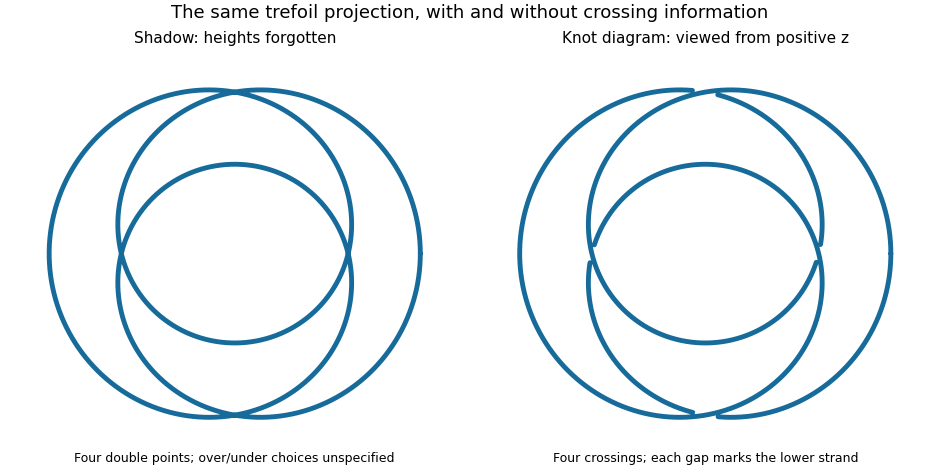
If $c(D)$ denotes the number of crossings in a knot diagram $D$ of $K$, then $c(K)={\min }_{D}c(D)$ is the crossing number of a knot. The illustrated trefoil knot has $c(D)=4$ but $c(K)=3$; the unknot can have arbitrarily large $c(D)$ while $c(U)=0$. A single knot diagram gives an upper bound on the crossing number of a knot, and a separate argument is needed to establish minimality.

A knot shadow is the curve in the Euclidean plane underlying a knot diagram after its overcrossing and undercrossing information has been erased. At a crossing the two local branches still continue across one another; the drawing does not specify which lies higher in space.

Knot theory studies closed curves in three-dimensional Euclidean space that cannot intersect themselves, and asks which can be deformed into one another without cutting or passing one strand through another. Its basic object is a knot: a smooth embedding of a circle, considered up to ambient isotopy. Several disjoint knots form a link. More generally, knot theory studies such embeddings in other manifolds and in higher dimensions.

The central surprise is that a flexible circle can carry permanent information about how it sits in space. A trefoil knot and an unknot each consist of just one circle, but no ambient isotopy turns one into the other. A knot diagram translates this spatial question into a finite drawing; Reidemeister moves describe the changes of drawing that preserve the knot. Knot invariants translate it into computations: unequal Alexander polynomials of a knot, Jones polynomials, or knot groups certify different knots. Equal values of a particular knot invariant generally leave the question open; even an isomorphism of knot groups alone is not a complete classification.

An early foundation for working with knot diagrams is Kurt Reidemeister's 1927 paper Elementare Begründung der Knotentheorie, published in volume 5 of Abhandlungen aus dem Mathematischen Seminar der Universität Hamburg, pages 24–32.^[ref] Marc Lackenby's authored notes Elementary knot theory, Section 2.4, explain the Reidemeister move theorem and its role in searching for a certificate that two knot diagrams represent the same knot.^[ref]

Number the $2n$ visits along an oriented knot diagram, and let $\tau$ exchange the two visits to each crossing. At an oriented smoothing, an incoming strand follows the outgoing strand of the other visit. Thus the cycles of the displayed permutation are exactly the Seifert circles. Their count $s$ gives the Seifert algorithm genus $(1-s+n)/2$ without requiring a separate drawing of the smoothed diagram.

False as written for arbitrary links. The two-component unlink has a diagram with no crossings butThe correct connected-diagram statement does hold, in particular for every knot diagram. If $s_A,s_B$ count the all-$A$ and all-$B$ bracket smoothing state circles, changing $j$ smoothings increases the circle count by at most $j$. The maximum and minimum $A$ exponents therefore lie between $n+2s_A-2$ and $-n-2s_B+2$. This gives the Kauffman bracket breadth bound ${\mathrm{br}}_A⟨D⟩\le 2n+2s_A+2s_B-4$. For a connected projection, the Turaev surface has Euler characteristic $s_A+s_B-n\le 2$, so the bound is $4n$. Writhe of a link diagram normalization changes only a monomial, and $t=A^{-4}$ divides the breadth by four, giving $\mathrm{br}{V}_L\le n$.

For a diagram with $k$ projection components, sum the same Euler characteristic inequality over the components. Then $s_A+s_B\le n+2k$ and the Jones polynomial breadth bound for a disconnected diagram is $\mathrm{br}{V}_L\le n+k-1$. The extra $k-1$ is indispensable, as the unlink shows.

We use $[a,b]=a^{-1}{b}^{-1}ab$. To obtain a Wirtinger presentation, choose an oriented regular knot diagram, cut its strands at undercrossings, and give each resulting arc a positively oriented meridian of a knot. The complement of the arcs above the projection plane has a free fundamental group on these meridians. At a crossing, pushing an understrand meridian past the overstrand conjugates it by the overstrand meridian. Thus, if $a$ is the overstrand generator and $b,c$ are the incoming and outgoing understrand generators, the relation is $c=a^{ϵ}b{a}^{-ϵ}$, where $ϵ$ is determined by the crossing orientation. Applying the Seifert-van Kampen theorem while adjoining the crossing neighborhoods gives one such relation per crossing. The remaining three-dimensional region adds no fundamental-group relation. For a connected diagram one crossing relation is redundant. This derives a group presentation from any tame knot diagram, rather than just specifying a recipe without its topological justification.

For the Borromean rings, choose three meridians $x,y,z$ and call the other three arc meridians $x^{\prime },y^{\prime },z^{\prime }$. Base paths and orientations can be chosen so the six crossing relations readEliminate the primed generators with the first row. The second row says respectively that $x$ commutes with $(z^{\prime }{)}^{-1}z=[y^{-1},z]$, that $y$ commutes with $(x^{\prime }{)}^{-1}x=[z^{-1},x]$, and that $z$ commutes with $(y^{\prime }{)}^{-1}y=[x^{-1},y]$. The last relation is redundant, just as one crossing relation is redundant in the Wirtinger presentation. Alternatively the Hall-Witt identity, after conjugating its three factors, shows that any two of these cyclic relations imply the third. Hence the Borromean link group isBoth relators have zero exponent sum in each generator. Passing from the free group to its abelianization therefore imposes no relations beyond commutation, andEquivalently the three linking-number maps to $\mathbb{Z}$ independently detect the three meridians.

Here is an explicit representation, followed by a faithfulness argument:Each determinant is one. Direct multiplication verifies the two relators. For example $[Y^{-1},Z]=\left(\begin{array}{cc}-1& 2i\\ 0& -1\end{array}\right)$, which commutes with $X$. Merely checking those relators would not prove faithfulness, so we identify the image's complete group presentation.

Write $B=PS{L}_2(\mathbb{Z}[i])$, the Gaussian Bianchi group, and use its four generators $T,U,L,A$ from the allowed presentation. In $B$ the three proposed generators areThe last equality is in $PS{L}_2$, so an overall minus sign in matrix multiplication is immaterial. Reduce matrices modulo $4$ in $\mathbb{Z}[i]$, and then quotient by $\{\pm I\}$. The finite image $Q$ has order $1536$: the residue field is ${\mathbb{F}}_2$, $S{L}_2({\mathbb{F}}_2)$ has order six, and each of the three subsequent local-ring layers has a kernel of order $2^3$, before the final quotient by $\{\pm I\}$. Elementary elimination over this local ring shows that the images of $T,U,A$ generate it. The subgroup $\bar{H}=⟨\bar{X},\bar{Y},\bar{Z}⟩$ has order $64$, as multiplication in this finite ring verifies. Let $K$ be its inverse image in $B$; then $[B:K]=24$.

For completeness the following gives the coset computation needed to check the subgroup presentation explicitly. Cosets are right cosets $Kr$; columns record right multiplication by $T,U,L,A$. Representatives are words in the allowed generators.Apply the Reidemeister–Schreier theorem: for a transition $j{⟶}^{g}k$, use generator $r_{j}g{r}_k^{-1}$, omitting the 23 tree transitions. Rewrite each of the eight allowed ambient relators starting at each of the 24 rows. There are 73 remaining Schreier generators. Adjoin the names $x=T$, $y=A{U}^{-2}{A}^{-1}$, $z=A{T}^{-2}{A}^{-1}L{U}^{-1}$ and eliminate the Schreier generators using relations in which they occur once. The remaining relations, with an uppercase letter denoting the inverse of the corresponding lowercase one, are the wordsThis table and the rewriting rule determine every relation without an appeal to a guessed presentation. In this notation cyclically reduced versions of the two desired relators are $r=ZYzXZyzYxy$ and $q$. Elementary substitutions of relator segments, with cyclic reduction at each step, giveusing $r,q$; conversely $r⟶p⟶1$ using $p,q$. These substitutions show equality of the two normal closures. For example the first substitution replaces $xyX$ in the cyclic rotation of $p$ by $zxZyzXZ$, as allowed by $q$, and then the initial $ZYz$ is replaced by $YXyZYzx$ using $r$. Thus $K$ has exactly the presentation of $G$, with $x,y,z$ represented by $X,Y,Z$. In particular these three matrices generate $K$, and

To identify the actual link complement as a hyperbolic three-manifold, rather than only on a manifold with an isomorphic group, cut along the projection-plane regions, making the usual small crossing detours above and below. The octahedral projection graph has eight triangular regions. The upper and lower pieces are ideal octahedra; corresponding faces are matched with one-third-turn corner permutations, with opposite directions on adjacent checkerboard faces. Reversing these cuts reconstructs the link complement. Give both pieces the regular ideal hyperbolic space octahedron metric. All triangular face maps are isometries and each edge cycle has four dihedral angles $\pi /2$, so the metric has no edge singularity. Equal horospherical truncations match in Euclidean squares and assemble into three flat tori, giving complete torus cusps. The compact truncated remainder and these cusps show completeness and finite volume. Thus the Borromean complement is a complete finite-volume hyperbolic three-manifold. This also supplies a geometric discrete faithful holonomy, independently of the subgroup calculation.

A Wirtinger presentation from a connected knot diagram has one generator per arc and one relator per crossing, with one relator redundant. Its presentation complex is a finite two-dimensional CW complex $X$ with one zero-cell, $n$ one-cells, and $n-1$ two-cells, and the usual diagrammatic construction gives a homotopy equivalence $X\simeq E_K$.

The abelianization of the knot group is $H_1(E_K;\mathbb{Z})\cong \mathbb{Z}$, generated by a meridian of a knot. Every homomorphism to the cyclic group $\mathbb{Z}/2$ factors through this abelianization, and reduction modulo two is its unique surjection. Thus the requested map $\alpha$ is unique.

Its kernel determines a two-sheeted covering space $\hat{X}$. The nontrivial deck transformation acts on cellular chains and homology, giving them module structures over the group ringLift one copy of every cell of $X$; its two deck translates form a free $\hat{R}$-basis. Hence $C_0\cong \hat{R}$, $C_1\cong {\hat{R}}^n$, and $C_2\cong {\hat{R}}^{n-1}$. If $\tilde{X}$ is the infinite cyclic cover, its cellular chains are free over $R=\mathbb{Z}[t^{\pm 1}]$, and imposing $t^2=1$ gives

For an odd prime $p$, the two idempotents $e_{+}=(1+t)/2$ and $e_{-}=(1-t)/2$ split the group algebraThe plus summand is the cellular chain complex of $X$ with ${\mathbb{F}}_p$ coefficients, while the minus summand is $C_{-}=C_{\ast }^{\mathrm{cell}}(\tilde{X}){\otimes }_R{R}_{-}$. Therefore

On the minus summand, the boundary $t-1:C_1\to C_0$ becomes multiplication by $-2$, which is invertible in ${\mathbb{F}}_p$, so $H_0(C_{-})=0$. After the corresponding cancellation, the remaining square boundary matrix is an Alexander matrix specialized at $t=-1$. It is singular over ${\mathbb{F}}_p$ exactly whenor equivalently when $p$ divides the knot determinant $\det K$. Thus $H_{\ast }(C_{-})$ is nonzero exactly in that case.

Finally, $\det K=|{\Delta }_K(-1)|$ is a nonzero odd integer, so the minus complex is acyclic over $\mathbb{Q}$. Since a knot exterior has the rational homology of a circle,

Apply the oriented smoothing to every crossing of an oriented knot diagram, fill the resulting Seifert circles by disjoint disks at suitable heights, and reconnect them by twisted bands at the original crossings. The boundary is the original knot. If the connected surface has $s$ disks and $c$ bands, its Euler characteristic is $s-c$ and its genus is $(1-s+c)/2$.

The trefoil is the torus knot $T_{2,3}$. It is the simplest nontrivial knot by crossing number of a knot: $c(T_{2,3})=3$. A standard three-crossing alternating knot diagram is reduced, so the Tait crossing-number theorem establishes minimality. The four-crossing knot diagram shown below also represents the trefoil knot, illustrating that a particular projection need not achieve that minimum. Its Seifert genus is one.

Here is a small algebraic certificate that a trefoil knot cannot be deformed into an unknot. One Seifert matrix for a trefoil knot isTaking the determinant gives the Alexander polynomial of a knotwhere $\doteq$ allows multiplication by a Laurent unit $\pm t^n$ in the Laurent polynomial ring. No such multiplication turns this three-term Alexander polynomial of a knot into the unknot's value $1$. Since the Alexander polynomial of a knot is a knot invariant, this computation rules out every possible ambient isotopy between the two knots; it does not merely rule out the deformations we happened to try.

The knot group supplies another certificate. The presentation $⟨a,b\mid a^2=b^3⟩$ maps onto the symmetric group $S_3$ by $a\mapsto (12)$ and $b\mapsto (123)$, since both sides of the relation map to the identity. These images generate a non-abelian group, so the knot group cannot be the unknot's infinite cyclic group. However, a trefoil knot and its mirror of a link have isomorphic knot groups: the abstract knot group alone does not distinguish all knots.

The unknot $U$ is the knot type represented by the planar circleEquivalently, an unknot is a knot that bounds a smoothly embedded disk in the three-sphere. The disk must itself be embedded; merely filling a loop with a map that is allowed to intersect itself does not establish that the knot is an unknot. Flattening a neighborhood of an embedded spanning disk explains why this criterion recovers the planar circle.

A complicated drawing can still represent an unknot. Starting with a crossing-free knot diagram of $U$, insert a small kink by a type I Reidemeister move. The resulting knot diagram has one crossing, but removing the kink exhibits the same unknot. Repeating in separate small regions gives knot diagrams of the unknot with arbitrarily many crossings, although the crossing number of a knot is $c(U)=0$. A drawing's apparent complexity is therefore not a certificate of knotting.

The normalized Alexander polynomial of a knot and Jones polynomial of the unknot are both $1$, and its knot group is the infinite cyclic group $\mathbb{Z}$, because the knot exterior is a solid torus. These are useful comparison values. In particular, a nonconstant Alexander polynomial of a knot certifies that a knot is not an unknot, but the converse fails: nontrivial untwisted Whitehead doubles also have Alexander polynomial of a knot $1$.