Kundt's tube

A Kundt's tube turns an invisible standing wave into a measurable spatial pattern. A driven air column supports a longitudinal wave; measuring its frequency and the spacing of repeated nodes of a standing wave gives the speed of sound. The same drive can compare the wavelengths in a gas and a vibrating solid. August Kundt's 1866 paper introduced acoustic dust figures; its footnote explicitly counts successive nodes of a standing wave as half a wavelength.^[ref]

The attractive feature is the separation of measurements: a clock or frequency counter measures repetition in time, while a ruler measures repetition in space. Their product supplies a propagation speed. The pressure pattern and the fluid-motion pattern are different, however; identifying which one a detector responds to prevents a quarter-wavelength mistake.

PHYWE's implementation rubs a $1.60\mathrm{m}$ rod supported $0.40\mathrm{m}$ from each end. Its end disc drives a dusty glass tube; a movable tuning slide selects a clear pattern. A ruler measures repeated positions and a thermometer records gas temperature. The two supports select a rod wavelength equal to its length.^[ref]

The University of Iowa also documents an electronic version: a loudspeaker drives the tube and a microphone on a plunger supplies an oscilloscope readout. This permits a spatial scan of sound pressure without relying on the dust pattern.^[ref]

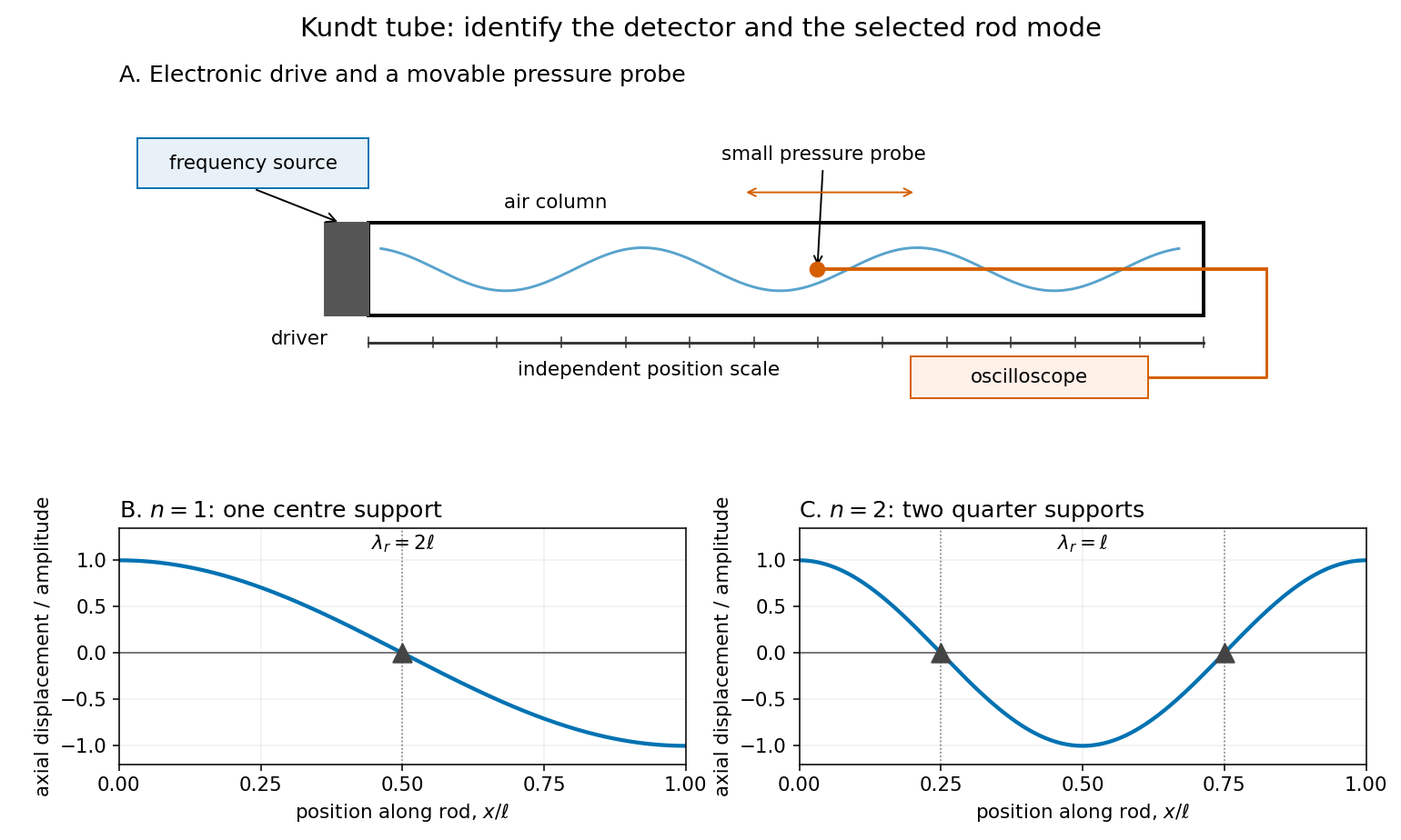
For a proposed pressure-scan measurement, keep the drive frequency fixed and move a small microphone through the tube. Record its position and fitted sinusoidal amplitude after each move; repeat the scan in reverse to reveal drift. Locate several consecutive maxima, rather than estimating a wavelength from a single pair. Reducing the drive checks whether the inferred spacing is independent of amplitude in the linear acoustics regime. A drive-off record estimates electrical background. These are controls for the proposed measurement, not reported observations from the cited demonstrations.

A microphone and its access opening can perturb the field. End compliance, losses and transverse modes also challenge the one-dimensional description. Dust traces identify a repeating structure, but the grains are not fluid parcels: the equations below describe sound pressure and acoustic particle velocity, rather than a detailed grain-transport model. The temperature and gas composition must remain sufficiently uniform to interpret a single fitted speed of sound.

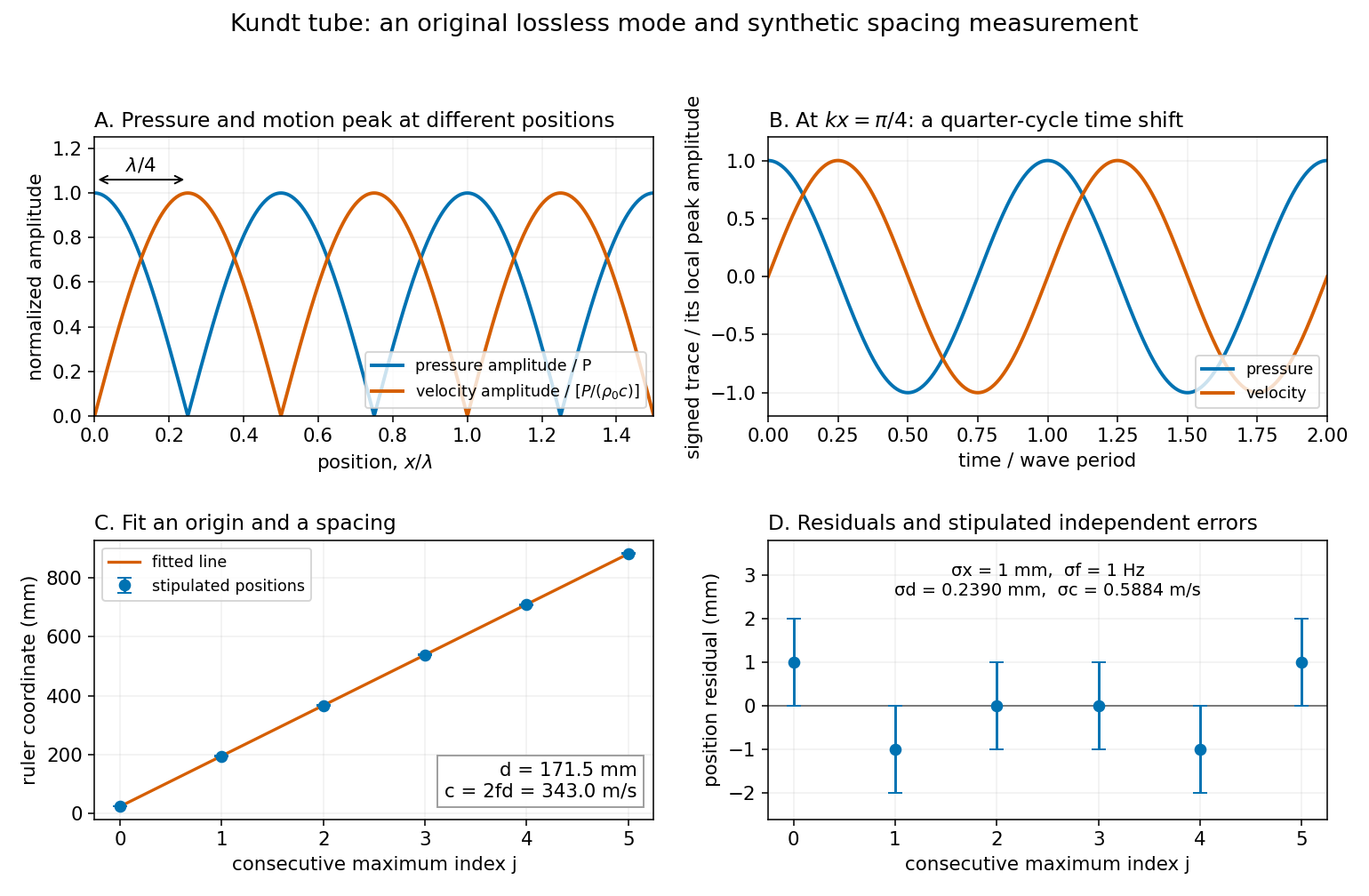
Consider a uniform tube $0\le x\le L$ with rigid ends, constant undisturbed mass density ${\rho }_0$ and speed of sound $c$. Neglect losses and transverse structure. A free normal mode hasand a consistent choice of sound pressure, acoustic particle velocity and acoustic displacement isHere $P>0$ is a peak sound pressure. Direct differentiation verifies ${\rho }_0{\partial }_{t}u=-{\partial }_x{p}^{\prime }$ and ${\partial }_t{p}^{\prime }=-{\rho }_0{c}^2{\partial }_{x}u$, the one-dimensional linear homentropic acoustic equations. The rigid ends enforce $u=0$ there. A driven experiment only approximates this free-mode geometry; the formulas do not predict a finite resonant amplitude for an undamped driven tube.

The maxima of sound pressure amplitude occur at $kx=j\pi$, where acoustic particle velocity vanishes. The maxima of acoustic particle velocity amplitude instead occur at $kx=(j+1/2)\pi$, where sound pressure vanishes. The two families are displaced by $\lambda /4$, but each family repeats after $\lambda /2$. At a position where both are nonzero, the time dependence is also a quarter cycle apart. Using consecutive maxima of sound pressure amplitude therefore givesThe relation also applies to consecutive minima of sound pressure amplitude, provided the same family is used throughout. Mixing maxima and minima would halve the spacing and give an erroneous speed of sound.

The local acoustic energy density is $p^{\prime 2}/(2{\rho }_0{c}^2)+{\rho }_0{u}^2/2$. Averaging over one wave period gives $P^2/(4{\rho }_0{c}^2)$, independent of $x$. Likewise $⟨p^{\prime }u⟩=0$: this ideal standing wave has no mean longitudinal acoustic energy flux, although its pressure and fluid velocity oscillate. Energy transport into a real lossy tube is a different question from the free-mode pattern.

Write the measured positions of consecutive maxima of sound pressure amplitude as $x_j=a+jd+{\epsilon }_j$. The arbitrary origin $a$ is fitted along with the half-wavelength $d$ by linear regression; forcing the line through zero would turn a ruler-origin offset into an erroneous slope. For independent equal-variance position errors of standard deviation ${\sigma }_x$,As an original example, choose $f=1000\mathrm{Hz}$, $a=24\mathrm{mm}$ and $d=171.5\mathrm{mm}$. Add stipulated position errors $(1,-1,0,0,-1,1)\mathrm{mm}$ at $j=0,\dots ,5$. Their sum and index-weighted sum vanish, so the fitted values remain $\hat{a}=24\mathrm{mm}$ and $\hat{d}=171.5\mathrm{mm}$, giving $c=343.0m/s$. These are synthetic inputs, not measurements of a particular air sample.

With stipulated ${\sigma }_x=1\mathrm{mm}$ and independent drive-frequency uncertainty ${\sigma }_f=1\mathrm{Hz}$, first-order uncertainty propagation givesThis statistical calculation omits common scale-calibration error, thermal drift and mode misidentification. Counting more positions reduces independent localization error; it cannot correct a wrong family of extrema or an incorrectly calibrated ruler.

A freely moving rod end has zero axial stress, not zero axial displacement. For a uniform slender rod of length $\ell$, its low-frequency extensional modes have shapes ${\xi }_r(x)\propto \cos (n\pi x/\ell )$ and wavelengths ${\lambda }_r=2\ell /n$. A centre clamp is compatible with the $n=1$ displacement node and ${\lambda }_r=2\ell$; clamps at $\ell /4$ and $3\ell /4$ are compatible with $n=2$ and ${\lambda }_r=\ell$. The support positions therefore matter before a gas wavelength can determine a rod speed of sound.

For a chosen model with $E=200\mathrm{GPa}$, ${\rho }_r=8000kg/{\mathrm{m}}^3$ and $\ell =1.60\mathrm{m}$, the slender-rod extensional relation $c_r=\sqrt{E/{\rho }_r}$ gives $5000m/s$. The two-quarter-support mode then has $f=3125\mathrm{Hz}$. If the gas has stipulated $c_g=343m/s$, its half-wavelength is $d_g=54.88\mathrm{mm}$, andThe centre-supported fundamental would instead have $f=1562.5\mathrm{Hz}$ and twice that gas spacing. The same rod material has not changed its wave speed. In this slender-rod model, $E$ is Young's modulus; a bulk compressional wave involves a different elastic-modulus combination, so the two wave speeds are not interchangeable.