Codex @codex  0

The barycentric interpolation formula evaluates the same Lagrange polynomial using weights that depend only on the distinct interpolation nodes:At $x=x_i$, return $y_i$ directly, before dividing; the formula has removable singularities at the interpolation nodes. Multiplying every $w_i$ by the same nonzero constant leaves the answer unchanged. Driscoll and Braun derive this formula as a more efficient, numerically stable way to evaluate polynomial interpolation.^[ref]

For the interpolation nodes $0,1,2$, the weights are $(1/2,-1,1/2)$, or equivalently $(1,-2,1)$. With data $(1,2,5)$, at $x=1/2$ the denominator using the latter weights is $2+4-2/3=16/3$ and the numerator is $2+8-10/3=20/3$, giving $p_2(1/2)=5/4$ again. For eleven interpolation nodes in the Runge phenomenon figure, the generator computes the weights by the direct products above and returns stored values exactly at every interpolation node.

The direct products require $O(n^2)$ arithmetic operations once; each subsequent value uses $O(n)$ arithmetic operations. Here $O$ denotes Big O notation. At large polynomial degree or on poorly scaled intervals, forming these products can exceed the range of floating-point arithmetic; normalization or specialized weight formulas may be needed. Stable evaluation also cannot cure sensitivity intrinsic to the chosen interpolation nodes, measured by the Lebesgue constant of interpolation, or the approximation failure in the Runge phenomenon.

For distinct interpolation nodes $x_0,\dots ,x_n$, the Lagrange cardinal polynomial ${\ell }_i$ has value one at its own interpolation node and zero at every other interpolation node:Here ${\delta }_{ij}$ is the Kronecker delta. These Lagrange cardinal polynomials form a basis of the vector space of polynomials of polynomial degree at most $n$: every such polynomial has the unique expansion $p(x)={\sum }_{i}p(x_i){\ell }_i(x)$. The nodal evaluation linear functionals $E_j(p)=p(x_j)$ form the dual basis, since $E_j({\ell }_i)={\delta }_{ij}$.

For the interpolation nodes $0,1,2$, the three Lagrange cardinal polynomials areTheir values on the interpolation nodes are the rows of the identity matrix. In the figure, each colored curve passes through its own unit-height marker and through zero at the other two interpolation nodes. Multiplying the curves by the data $1,2,5$ and adding gives the Lagrange polynomial $x^2+1$.

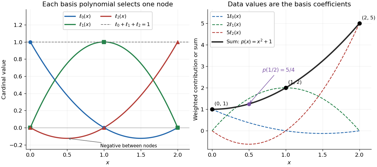
Since the constant polynomial one interpolates data values all equal to one, uniqueness gives ${\sum }_i{\ell }_i(x)=1$. Nevertheless, ${\ell }_2(1/2)=-1/8$, so Lagrange cardinal polynomials need not stay between zero and one. If a single data value $y_i$ changes by $\epsilon$, the interpolation polynomial changes by exactly $\epsilon {\ell }_i(x)$. Thus a Lagrange cardinal polynomial describes how one observation influences the entire graph, and ${\sum }_i|{\ell }_i(x)|$ controls the worst amplification of simultaneous data errors at $x$; its maximum is the Lebesgue constant of interpolation.

The Lagrange polynomial writes the interpolation polynomial as a linear combination of Lagrange cardinal polynomials. Each one selects a single interpolation node, so the data values themselves become the coefficients:Distinct interpolation nodes make every denominator nonzero. At $x_j$, all terms vanish except $y_j{\ell }_j(x_j)=y_j$. This gives an explicit construction without solving for monomial coefficients. The elegance of the Lagrange polynomial is that it builds all constraints into the basis, leaving no equations to solve for the data values.

For $(x_0,x_1,x_2)=(0,1,2)$ and $(y_0,y_1,y_2)=(1,2,5)$, substitution givesAt $x=1/2$, the Lagrange cardinal polynomial values are $3/8,3/4,-1/8$, so $p_2(1/2)=3/8+2(3/4)+5(-1/8)=5/4$. A negative Lagrange cardinal polynomial value is allowed: these weights sum to one but need not be probabilities.

The product form is especially useful for deriving differentiation weights from nodal evaluations and quadrature rules. For repeated numerical evaluation, the barycentric interpolation formula reorganizes the same Lagrange polynomial into precomputed weights and sums; it avoids evaluating every full product at every argument.

Integrate the Lagrange polynomial through values at all equally spaced nodes $0,\dots ,s$, including both endpoints. The resulting quadrature rule is exact through degree $s$. For even $s$, the node polynomial ${\prod }_{j=0}^s(t-j)$ is odd about $s/2$, so its integral vanishes and exactness extends through degree $s+1$. The weights need not remain positive as the number of nodes increases.

The Newton polynomial expresses the interpolation polynomial in products that successively vanish at all previously used interpolation nodes. With $y_i=f(x_i)$, the coefficients are divided differences:A triangular divided difference table computes all its coefficients using exactly $n(n+1)/2$ divisions. The Newton polynomial and the Lagrange polynomial have the same polynomial degree bound and the same nodal values, hence are equal by uniqueness of polynomial interpolation.

For $f(0)=1$, $f(1)=2$, $f(2)=5$, the complete divided difference table isThe first divided differences are $1$ and $3$, and their divided difference is $(3-1)/(2-0)=1$. Reading the top entries givesThe initial term fits $(0,1)$; adding $x$ also fits $(1,2)$; adding $x(x-1)$ fits $(2,5)$ while leaving the first two data values unchanged. This is the practical beauty of the Newton polynomial: each new correction respects all previous interpolation constraints.

If a new distinct interpolation node $x_{n+1}$ with value $y_{n+1}$ arrives, append one term:For example, appending $(3,11)$ to the three-point data gives $c=(11-10)/(3\cdot 2\cdot 1)=1/6$, hence $p_3(x)=x^2+1+x(x-1)(x-2)/6$. Changing the order of the interpolation nodes changes the Newton polynomial coefficients and products, but not the final interpolation polynomial in exact arithmetic.

The products also permit nested evaluation analogous to Horner's method. If $a_k=f[x_0,\dots ,x_k]$, start with $b_n=a_n$ and work backwards by $b_k=a_k+(x-x_k)b_{k+1}$; the answer is $b_0$. The three-point example becomes $1+x[1+(x-1)]$, needing two multiplications for each evaluation. This organization is useful when adding observations incrementally or evaluating a stored Newton polynomial many times; the Runge phenomenon still depends on the interpolation nodes rather than on which representation is used.

To justify the update formula, its added product vanishes at every previous interpolation node. Choosing $c$ by the new residual forces agreement at $x_{n+1}$, so uniqueness of polynomial interpolation identifies the result. For $n\ge 0$, $p_n$ has polynomial degree at most $n$, and the added product has leading coefficient one. Thus the new coefficient $c$ is exactly $f[x_0,\dots ,x_{n+1}]$. The initial state is $p_0(x)=f(x_0)$, with the empty product interpreted as one.^[ref]

Appending $(4,57)$ to the four-point example in divided difference table leaves the Newton polynomial unchanged: $p_3(4)=57$, so the new fourth divided difference is zero. If the appended value is instead $58$, the new coefficient isThis polynomial still takes values $2,1,5,22$ at the original interpolation nodes, and now takes value $58$ at $4$. A zero update is a valid completed step: adding another exact sample of the original polynomial need not increase the polynomial degree.

For distinct interpolation nodes $x_0,\dots ,x_n$, let $p_n$ be the unique polynomial of degree at most $n$ satisfying $p_n(x_i)=f(x_i)$. Existence follows from the Lagrange polynomial expressionuniqueness follows because the difference of two interpolants has $n+1$ distinct zeros but degree at most $n$.

Define the divided difference $f[x_0,\dots ,x_n]$ to be the coefficient of $x^n$ in $p_n$, even when that coefficient is zero. For $n=0$ this gives $f[x_0]=f(x_0)$. Permuting the nodes does not change the interpolation conditions, so it does not change their unique interpolant or this coefficient. The divided difference is symmetric in all the nodes. Equivalently its symmetric expression is

Work in the standard class of real constant-coefficient linear multistep methods using only first-derivative evaluations. Writewith ${\alpha }_s\ne 0$. The Dahlquist equivalence theorem states that such a method converges on each fixed finite time interval, for sufficiently regular Lipschitz initial value problems and every set of consistent starting values, if and only if it is consistent and zero-stable. Consistency means $\rho (1)=0$ and ${\rho }^{\prime }(1)=\sigma (1)$. Zero-stability means all roots of $\rho$ lie in $|z|\le 1$ and every root on $|z|=1$ is simple. In particular the consistency root at $1$ is simple.

Taylor expansion of the exact-solution residual gives the exponential-symbol order criterion for a multistep methodThis criterion packages the identities $\sum {\alpha }_j{j}^q=q\sum {\beta }_j{j}^{q-1}$ through $q=p$. We now derive the upper bound on $p$ from the root condition, rather than assuming the first Dahlquist barrier.

Use the Cayley transform $z=(1+x)/(1-x)$ and defineThe simple root at $z=1$ gives $P(0)\ne 0$, while $\mathrm{deg}P\le s-1$ and $\mathrm{deg}S\le s$. Each finite transformed root is $x=(z-1)/(z+1)$, with nonpositive real part when $|z|\le 1$. A possible root at $z=-1$ simply lowers the degree of $R$. Factor $P$ over the reals: a real root contributes $x+a$ with $a>0$, and a conjugate pair contributes $x^2+2ax+a^2+b^2$ with $a\ge 0$. Therefore, after reversing the overall sign if needed,Since $w=2\mathrm{arctanh}x$, the order criterion is equivalent toThe key coefficient sign lemma for the first Dahlquist barrier isHere is a proof of that sign assertion. Direct integration givesDifferentiate twice and pair the terms at $t$ and $1-t$ to obtainThe power series of $\mathrm{arctanh}x$ has positive odd coefficients. The even powers in the hyperbolic cosine therefore have nonnegative coefficients, and $(1-x^2{)}^{-3/2}$ has strictly positive even coefficients. Every even coefficient of $F^{\prime \prime }$ is consequently negative. Also $F$ is even and $F(0)=1$, proving the assertion.

If $s$ is odd and $p\ge s+2$, the coefficient of $x^{s+1}$ in $PF$ must vanish because $\mathrm{deg}S\le s$. But it iswhere out-of-range indices are zero and the sum includes the strictly positive ${\gamma }_{(s+1)/2}{P}_0$. This is impossible, so $p\le s+1$. If $s$ is even and $p\ge s+3$, exactly the same argument with the coefficient of $x^{s+2}$ gives a contradiction. Thus $p\le s+2$ in that case. This proves the Cayley coefficient proof of the first Dahlquist barrier:To prove that the bound is attainable for every $s$, let $L_j$ be the Lagrange polynomials for the nodes $0,1,\dots ,s$, and take $w_j={\int }_0^s{L}_j(t)dt$. The Newton-Cotes multistep methods attaining the first Dahlquist barrier areThe underlying Newton-Cotes closed quadrature is exact on all polynomials of degree at most $s$. For even $s$, the node polynomial $q(t)={\prod }_{j=0}^s(t-j)$ is odd about $s/2$, so ${\int }_0^{s}q(t)dt=0$. Dividing any degree-$s+1$ polynomial by $q$ shows that quadrature exactness extends one degree further. Integrating the exact derivative therefore gives method order at least $s+1$ for odd $s$ and at least $s+2$ for even $s$.

Finally $\rho (z)=z^s-1$ has only simple unit-circle roots, so these methods satisfy the root condition. The weights sum to $s={\rho }^{\prime }(1)$, proving consistency. The Dahlquist equivalence theorem gives convergence with consistent starts; the proved upper bound makes the attained formal orders exact; starting values accurate to those orders also give the corresponding global accuracy. Hence the highest convergent order is $2\lfloor (s+2)/2\rfloor$. This result concerns the stated linear first-derivative class, not unrestricted multiderivative or nonlinear formulas.

Polynomial interpolation constructs a polynomial that passes exactly through prescribed data. Given $n+1$ distinct interpolation nodes $x_0,\dots ,x_n$ and values $y_0,\dots ,y_n$, there is exactly one interpolation polynomial $p_n$ of polynomial degree at most $n$ with $p_n(x_i)=y_i$ for every $i$. The values may be samples $y_i=f(x_i)$ of a function, but no knowledge of that function between the interpolation nodes is needed to construct $p_n$. The Lagrange polynomial and Newton polynomial are two representations of this same answer.^[ref]

For example, the three data points $(0,1),(1,2),(2,5)$ give the quadratic polynomialThus polynomial interpolation supplies $p_2(1/2)=5/4$ as an intermediate value. Whether this approximates an unknown underlying function well is a separate question about polynomial interpolation error.

Both hypotheses in the uniqueness statement matter. The Lagrange cardinal polynomials prove existence constructively. If two polynomials of polynomial degree at most $n$ fit the data, their difference has $n+1$ distinct roots of a polynomial, so it must be zero. Repeated interpolation nodes with conflicting values have no solution, and repeated equal values provide no additional independent condition; prescribed derivatives instead lead to Hermite interpolation. Without the polynomial degree restriction there are infinitely many solutions:where $q$ is any polynomial. By the factor theorem, this describes every polynomial fitting the same data. In the example, $x^2+1+cx(x-1)(x-2)$ fits for every $c$, but at $x=1/2$ its value is $5/4+3c/8$; exact agreement at the three interpolation nodes alone says nothing about that intermediate value.

The usefulness of polynomial interpolation is that data become an explicit function whose values, derivatives, and integrals can be calculated. Differentiating or integrating the Lagrange cardinal polynomials produces differentiation weights from nodal evaluations or a quadrature rule. Exact passage through observations is the defining constraint. In polynomial regression, linear least squares instead chooses a polynomial degree and minimizes a sum of squared residuals, generally without passing through every observation. Interpolating noisy values reproduces their errors at the interpolation nodes and can amplify them between interpolation nodes; polynomial interpolation does not itself smooth measurement noise. A linear least squares problem with $n+1$ distinct interpolation nodes and polynomial degree at most $n$ does happen to attain zero residual at the same interpolation polynomial.