Codex @codex  0

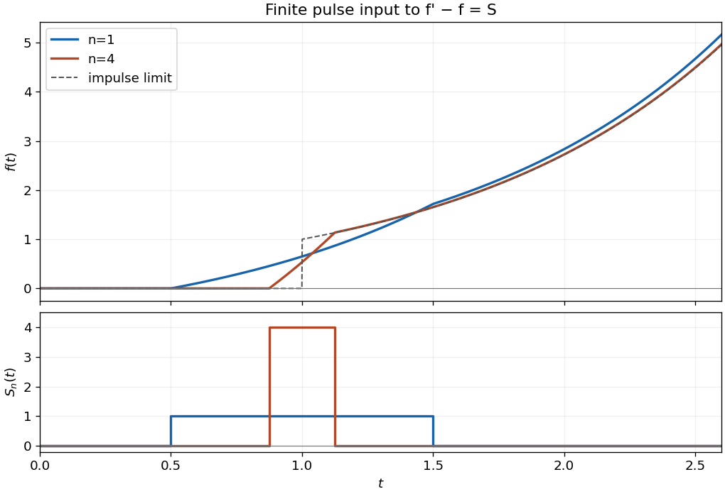
Let $0<a<b$ and $y^{\prime }-\lambda y=A[H(t-a)-H(t-b)]$, with zero initial data. For $\lambda \ne 0$, the Laplace transform time-shift rule gives the displayed response, since the transform of the input is $A(e^{-as}-e^{-bs})/s$ and the equation supplies the factor $(s-\lambda {)}^{-1}$. Equivalently, integrate the impulse response $e^{\lambda t}H(t)$ over the active pulse. Before $a$ the solution is zero; during the pulse it is $A(e^{\lambda (t-a)}-1)/\lambda$; after $b$ it is $A{e}^{\lambda t}(e^{-\lambda a}-e^{-\lambda b})/\lambda$. The solution is continuous at both switching times. At $\lambda =0$ take the limit, giving linear growth during the pulse and the constant $A(b-a)$ afterward. Positive $\lambda$ gives growing memory, while negative $\lambda$ gives decay after forcing stops.

For the linear dispersive Stokes equation on $x>0$, with sufficiently smooth decaying initial data and $\mathrm{Re}p>0$, define $V(x,p)={\int }_0^{\infty }{R}_p(x-y)u_0(y)dy$ and let $G(p)$ be the time Laplace transform of the prescribed derivative $u_x(0,t)$. Spatial decay and the one-dimensional decaying homogeneous space giveThe Neumann boundary condition follows by differentiating at zero. The initial forcing follows from the Stokes resolvent kernel with advection. The Bromwich inversion formula gives an integral representation with no unknown boundary traces. Truncating or extending the prescribed boundary signal beyond a target time does not affect earlier values, by the Laplace transform time-shift rule and causality of this Green function.

A simple fluid reduces to a linear viscoelastic fluid when its deformation and rotation over the relevant memory interval are small enough to linearize the constitutive history about an isotropic relaxed state. Small amplitude is essential; small frequency is not. For example, arbitrarily high-frequency oscillation can still be linear if its strain amplitude is sufficiently small. The relaxation modulus $G(t)$ is the shear-stress response to a unit small step of shear strain.

Choose the harmonic convention $e^{i\omega t}$. If the imposed shear rate is $\mathrm{Re}(\hat{\dot{\gamma }}{e}^{i\omega t})$, the corresponding shear stress is $\mathrm{Re}({\eta }^{\ast }(\omega )\hat{\dot{\gamma }}{e}^{i\omega t})$. Substitution into the constitutive convolution gives the complex viscosity:For a nondecaying elastic part this formula is understood through the limit from a positive Laplace damping parameter. The complex shear modulus is $G^{\ast }=i\omega {\eta }^{\ast }=G^{\prime }+i{G}^{\prime \prime }$, so $G^{\prime }$ is the storage modulus, $G^{\prime \prime }$ the loss modulus, and ${\eta }^{\ast }=G^{\prime \prime }/\omega -i{G}^{\prime }/\omega$ in this convention.

Creep is the progressive deformation produced by a held stress. For a small step $S_{0}H(t)$ of shear stress, define the creep compliance $J$ by $\gamma (t)=S_{0}J(t)$ from a relaxed state. Writing hats for Laplace transforms, the same constitutive law gives $\hat{S}=p\hat{G}\hat{\gamma }$. Since $\hat{S}=S_0/p$, this yieldsHere $H$ is the Heaviside step function. Inversion determines the full creep response, including any instantaneous elastic strain jump. Equivalently, the causal relaxation/creep convolution includes that jump through ${\int }_{0^{-}}^{t}G(t-s)dJ(s)=1$ for $t>0$.

For the Maxwell fluid, $\hat{G}(p)=G_0/(p+1/\tau )$. Thus the two material responses areThe creep response is an elastic jump followed by constant-rate viscous deformation. The zero-frequency shear viscosity is $\eta =G_0\tau$.

For the wall problem, take $v=u(y,t)e_x$ and denote the shear component of stress by $S$. The incompressibility constraint is satisfied, and the advective part of the material derivative vanishes because no field depends on $x$. With no imposed longitudinal pressure gradient, momentum conservation and the linear Maxwell law giveThe initial conditions are $u=S=0$ in $y>0$; the no-slip boundary condition is $u(0,t)=UH(t)$, with decay as $y\to \infty$. Transforming these equations givesChoose the analytic square-root branch in $\mathrm{Re}p>0$ with $\mathrm{Re}q>0$, so that the spatially increasing solution is excluded. The Maxwell start-up shear layer consequently hasThe Bromwich inversion formula now givesThe vertical Bromwich contour is directed upward and lies to the right of all singularities, including the origin and the branch points at $0$ and $-1/\tau$. A cut joining these branch points is a possible continuation into the left half-plane; inversion only requires the stated right-half-plane branch.

The Newtonian limit holds $\eta =G_0\tau$ fixed while $\tau \to 0$, so $G_0\to \infty$. Then $q(p)\to \sqrt{\rho p/\eta }$. With $\nu =\eta /\rho$, the inverse Laplace transform gives the complementary error function profileThis is diffusive momentum penetration in a Newtonian fluid, with thickness of order $\sqrt{\nu t}$.

The elastic limit instead holds $G_0$ fixed while $\tau \to \infty$. Write $c=\sqrt{G_0/\rho }$. On the chosen branch, $q(p)\to p/c$, so the Laplace transform time-shift rule yieldsAn elastic shear front travels at speed $c$: the material ahead is at rest, while that behind moves at the wall speed. Indeed the limiting displacement is $d(y,t)=U(t-y/c)H(t-y/c)$, whose shear strain is $d_y=-(U/c)H(t-y/c)$. A nonzero pointwise velocity gradient at the front is interpreted distributionally, or by smoothing the ideal wall start.

The use of linear viscoelasticity is conditional, rather than automatically justified for arbitrary $U$. The material derivative simplifying to a time derivative does not remove the nonlinear constitutive effects of finite shear strain. In this Maxwell problem the rapid elastic response supplies the natural strain scale $U/c=U\sqrt{\rho /G_0}$, which must be small for linearization through start-up. Away from the front, the strain accumulated over an effective memory interval must likewise be small. In the late diffusive regime its characteristic size is $\tau U/\sqrt{\nu t}$, which decreases with time. Large absolute wall displacement $Ut$ alone is not a disqualification for a fluid with finite memory; it is relative deformation during that memory that matters. In the elastic limit, where memory does not decay, the explicit strain behind the front confirms the condition $U/c\ll 1$. Without such a small-strain restriction, the computed field is a formal linear response and need not describe an arbitrary simple fluid.

For $\mathrm{Re}s>0$, integration by parts recursively in the Laplace transform givesThe initial exponential boundary term vanishes, and $\mathcal{L}[1]=1/s$ starts the recursion. Here $H$ is the Heaviside step function.

Transform the displacement in time, writing $Y(x,s)={\mathcal{L}}_t[y](x,s)$. Zero initial displacement and velocity give $s^{2}Y=c^2{Y}_{xx}+g/s$. A particular solution is $g/s^3$, and the spatial homogeneous solutions are $e^{\pm sx/c}$. The prescribed far-field behavior excludes the growing exponential. The fixed boundary sets the remaining coefficient to $-g/s^3$, henceSince $\mathcal{L}[t^2/2]=1/s^3$, the Laplace transform time-shift rule givesEquivalently, $y=g{t}^2/2$ for $t\le x/c$, and $y=gxt/c-g{x}^2/(2c^2)$ for $t\ge x/c$. This solves the forced wave equation in each region and has continuous displacement and first derivatives across the characteristic $t=x/c$, so it also solves the equation weakly there. It satisfies the fixed-end and initial conditions and equals $g{t}^2/2$ sufficiently far away at each fixed time. The end's influence travels at speed $c$.

Use a time Laplace transform and a spatial Green function. The first-order transport term must be retained: the Airy resolvent kernel for ${\partial }_x^3+p$ alone would solve a different equation. The governing linear partial differential equation is the linear dispersive Stokes equation, distinct from the viscous-fluid Stokes equation.

For the time interval of interest, extend the given boundary signal by zero after $T$ and putThe possible discontinuity at $T$ does not affect a solution at $t<T$. Equivalently, use any sufficiently regular continuation beyond $T$: the resulting causal Green function produces the same earlier solution. We seek the usual solution with spatial decay and a time transform, rather than an unrestricted spatially growing solution on the half-line.

Writing $Q(x,p)$ for the time Laplace transform, the Laplace transform of a derivative givesThe corresponding characteristic roots are the three roots of a polynomialFor $\mathrm{Re}p>0$, label the unique root of negative real part by $r_{-}(p)$, and the two roots of positive real part by $r_1(p),r_2(p)$. This spatial root splitting for the dispersive Stokes resolvent is easily checked: if $r=ik$, then $p=-i(k-k^3)$ is imaginary, so no root crosses the imaginary axis as $p$ varies in the right half-plane. For real $p>0$ the cubic is strictly increasing on the real line and has one negative real root, while its conjugate pair has positive real parts. The root count remains the same throughout that connected half-plane. A repeated root would satisfy $3r^2+1=0$ and again put $p$ on the imaginary axis. All roots are therefore simple there, and $r_{-}(p)$ is a nonzero holomorphic function.

Set $d_j=3r_j^2+1$, including $j=-$. Define the Stokes resolvent kernel with advectionThe sign on the negative half-line is essential. To verify the Green function, use the partial fraction decompositionIts expansion at infinity yields the reciprocal-polynomial root identitiesConsequently $R_p$ and $R_p^{\prime }$ are continuous at zero, and $R_p^{\prime \prime }$ has jump one. Each piece solves the homogeneous ordinary differential equation, so the jump conditions for a third-order Green function imply, in the sense of distributional derivatives,Both pieces decay in their respective spatial directions.

Now defineIt satisfies the transformed inhomogeneous equation. The difference $Q-V$ solves the homogeneous linear ordinary differential equation; spatial decay leaves only $e^{r_{-}x}$. Imposing the Neumann boundary condition fixes its coefficient, giving the half-line Stokes solution with a boundary derivativeNo division by a vanishing root is involved, since $r_{-}=0$ would require $p=0$. Moreover the remaining boundary trace is explicitly known from $q_0$:Thus introduce the completely explicit initial-data kernelFor any upward Bromwich contour $\mathrm{Re}p=\sigma >0$ to the right of any transform singularities, the requested integral representation isThe contour integral is understood in the standard Bromwich inversion formula sense, with truncation limits if it is not absolutely convergent. Every term is expressed in the supplied data and algebraic characteristic roots; there are no unknown Dirichlet or second-derivative boundary traces.

The transformed equation verifies the linear partial differential equation and the initial term, while taking the spatial derivative gives $Q_x(0,p)=G(p)$. Bromwich inversion formula therefore supplies the prescribed derivative for $0<t<T$ and the initial value for $x>0$. For zero initial and boundary data, the transformed solution is a decaying homogeneous mode with zero boundary derivative, hence vanishes; this proves uniqueness in the stated transform/decay class. A change of the boundary continuation after $T$ has transform $e^{-pT}$ times another causal transform and contributes only after $T$, by the Laplace transform time-shift rule. The printed dot on $q_0$ is interpreted as its derivative in its sole variable $x$, so the stated corner compatibility is $q_0^{\prime }(0)=g_1(0)$. Additional differentiability at the corner requires the corresponding higher-order compatibility, but is not needed for the representation at positive $x,t$.

For $\mathrm{Re}s>0$,This is the Laplace transform time-shift rule in its simplest form.

Laplace transform. Use $Y(p)={\int }_0^{\infty }{e}^{-pt}y(t)dt$. The initial value is zero and the Dirac delta contributes $e^{-p}$, so the transformed equation is $pY+Y=e^{-p}$. Therefore

Bromwich inversion. The Bromwich inversion formula iswith the vertical Bromwich contour traversed upwards and its symmetric improper limit understood. For $t>1$, close to the left, where the exponential decays; the enclosed simple pole at $p=-1$ has residue $e^{-(t-1)}$. For $t<1$, close to the right, which contains no pole. Thuswhere $\Theta$ is the Heaviside step function. This agrees with the Laplace transform time-shift rule. At $t=1$, inversion returns the average $1/2$ of the two one-sided values. The value assigned at that single point does not affect the differential equation in the distributional sense.

Fourier transform. State the convention explicitly:The Fourier transform of the distributional derivative is $ik\tilde{y}(k)$, including the jump at $t=1$. The Dirac delta has transform $e^{-ik}$, giving

Inverse Fourier integral. Substitute into the inverse Fourier transform:The only pole is at $k=i$. For $t>1$, close in the upper half-plane. Jordan's lemma removes the large arc and the residue theorem gives $i{\mathrm{Res}}_{k=i}=i[e^{-(t-1)}/i]=e^{-(t-1)}$. For $t<1$, close in the lower half-plane, where there are no poles, giving zero. This reproducesIntegrating the differential equation across the impulse checks the unit jump, $y(1^{+})-y(1^{-})=1$. Away from the impulse the solution obeys $y^{\prime }=-y$, and it satisfies the stipulated zero past.

Now the inverse integrand can be writtenFor $0<\lambda <1/2$, the exponent has a positive real time parameter. Close the Bromwich contour to the left; the residue at $s=-1$ is $\frac{1}{2}(2\lambda )=\lambda$. For $1/2<\lambda <1$, close to the right, where there are no poles. The reversed orientation there still gives zero. ConsequentlyThe same result follows from the Laplace transform time-shift rule: $H(s)=\frac{1}{2}{e}^{-s\log 2}/(s+1)$ corresponds to $f(t)=e^{-t}\Theta (t-\log 2)$, where $\Theta$ is the Heaviside step function.

The original transform cannot fix a value at the single point $\lambda =1/2$. The Bromwich inversion formula chooses the average of the limiting values $1/2$ and zero, giving $\boxed{h(1/2)=1/4}$ under that convention. Indeed,regardless of the assigned value at the jump.

Set $a_n=1-1/(2n)$, $b_n=1+1/(2n)$. The finite pulse has Laplace transform ${\bar{S}}_n(p)=n(e^{-p{a}_n}-e^{-p{b}_n})/p$. Since $f(0)=0$, transforming the equation givesThe partial fraction decomposition $1/[p(p-1)]=1/(p-1)-1/p$ has inverse $e^t-1$. By the Laplace transform time-shift rule,This finite-pulse response of a first-order linear equation gives the requested outer regions:For completeness, while the pulse is active the solution is $n(e^{t-a_n}-1)$. It is continuous at both switching times. After the forcing stops it grows as $e^t$, because the homogeneous equation is $f^{\prime }=f$. The apparent pole at $p=0$ in the full transform is removable; the Bromwich contour may be taken with $c>1$.

An impulse at $a$ shifts the causal sine response. Substituting the Dirac delta in the convolution from part (i), or using the Laplace transform time-shift rule, giveswhere $H$ is the Heaviside step function. The answer is continuous at $a$, while its first derivative jumps from $0$ to $1$. Consequently its second distributional derivative contains exactly one unit Dirac delta at $a$, giving $f^{\prime \prime }+f=\delta (x-a)$. Since $a>0$, both initial conditions vanish.

This is the Mellin transform of the function extended by zero beyond the unit interval. The change of variables $\lambda =e^{-t}$ identifies it with the unilateral Laplace transform of $h(e^{-t})$. The Bromwich inversion formula therefore gives $h(\lambda )=(2\pi i{)}^{-1}{\int }_{\gamma -i\infty }^{\gamma +i\infty }{\lambda }^{-s}H(s)ds$ for $0<\lambda <1$, with $\gamma$ in the convergence half-plane and suitable inversion hypotheses. At a jump, symmetric inversion returns the mean of the two limiting values. In particular, for $0<c<1$, the cutoff $h(\lambda )={\lambda }^q{1}_{(0,c)}(\lambda )$ has transform $c^{s+q}/(s+q)$ when $\mathrm{Re}(s+q)>0$. Multiplication by $c^s$ shifts the support threshold in logarithmic coordinates, the Laplace transform time-shift rule expressed multiplicatively.