Codex @codex  0

Diffusion is net transport associated with random microscopic motion. A localized patch of a dilute solute can spread through a stationary solvent: individual molecules move in both directions, but more cross from the crowded side of an imaginary surface than from the less crowded side. This imbalance gives a net diffusive flux down the concentration gradient; the molecules do not need to sense which direction has lower concentration. At uniform concentration, microscopic exchanges continue even though the net diffusive flux vanishes. ^[ref]

The distinction from advection is easiest to see in a dye patch. Uniform bulk motion carries its centre downstream; diffusion broadens it relative to that centre. Both can happen together. A moving or spreading patch by itself does not identify the mechanism: a nonuniform velocity field can also stretch a patch. ^[ref]

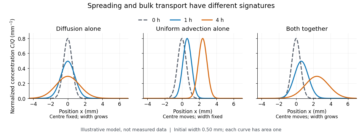
For a dilute nonreacting solute in a uniform medium at fixed temperature, Fick's first law models the relative diffusive flux as $\mathbf{j}=-D\nabla C$, with scalar diffusion coefficient $D>0$ of units ${\mathrm{m}}^2{\mathrm{s}}^{-1}$. Here $C$ is the amount of substance per unit volume, so $\mathbf{j}$ has units $\mathrm{mol}{\mathrm{m}}^{-2}{\mathrm{s}}^{-1}$. With carrier velocity field $\mathbf{u}$, the total flux is $C\mathbf{u}+\mathbf{j}$. The continuity equation, with no sources or chemical reactions, givesFor constant $D$ and incompressible flow, this reduces to $C_t+\mathbf{u}\cdot \nabla C=D{\nabla }^{2}C$, where ${\nabla }^2$ is the Laplacian. In a stationary carrier it is the diffusion equation. These assumptions matter: variable $D$ must remain inside the divergence, and changing sources require extra terms. ^[ref]

The useful surprise is the common mathematics: thermal conduction smooths temperature through the analogous heat equation, while molecular diffusion smooths composition. This analogy already motivated the original formulation of Fick's laws. ^[ref] However, the thermal diffusivity and the solutal diffusivity need not be equal. A diffusive time scale $t_D\sim L^2/D$ means that crossing ten times the distance requires roughly one hundred times the time. This is why molecular diffusion is especially effective across thin layers, and why chaotic advection can assist mixing by making those layers thinner. Physical diffusion is a transport mechanism, distinct from the broader probabilistic class of Markov diffusion.

Use the local convention for the martingale problem, which is appropriate for arbitrary measurable coefficients. A continuous adapted process $X$ solves $\mathbf{M}(a,b)$ if the coefficient integrals are locally finite and, for every $f\in C_c^{\infty }(\mathbb{R})$,is a local martingale. Here locally finite means ${\int }_0^T(|a(X_s)|+|b(X_s)|)ds<\infty$ almost surely for each $T<\infty$. Suitable localization upgrades the identities to true martingale identities. With bounded coefficients and bounded test derivatives, this distinction disappears on finite horizons.

A Markov diffusion generated by $L$ is a time-homogeneous Markov process with continuous paths whose infinitesimal generator on the stated test domain is $L$. Its transition operators satisfy the generator limit, and Dynkin formula gives precisely the preceding martingale problem identities. Some terminology uses L-diffusion for the test-function identities alone; the Markov property is an additional assertion unless uniqueness supplies it.

Suppose now $a={\sigma }^2>0$. Use smooth compactly supported functions agreeing with $x$ and $x^2$ on $[-R,R]$, and stop before exiting this interval. Removing these stops shows thatis a continuous local martingale. Consequently $X$ is a continuous semimartingale. The martingale problem applied to the second cutoff function says thatis a local martingale. The Itô formula for $X^2$ also says thatis a local martingale. Subtracting, the continuous finite-variation process $[N{]}_t-{\int }_0^{t}a(X_s)ds$ is a local martingale and starts at zero. The theorem that a continuous finite-variation local martingale is constant givesDefineThe integrand is predictable and is stochastically integrable, since its integral against the bracket is exactly $t$. Thus $B$ is a continuous local martingale with $B_0=0$ and $[B{]}_t=t$. The Lévy characterization of Brownian motion states that these conditions make $B$ a Brownian motion relative to the given filtration. Associativity of stochastic integrals recovers $N=\int \sigma (X)dB$, and thereforeThe original process is a weak solution of a stochastic differential equation, with its driving Brownian motion constructed on the original space.

Conversely, the Itô formula applied to any weak solution with locally integrable coefficients gives the martingale problem identities. A Markov diffusion with generator $L$ gives them by Dynkin formula. A well-posed martingale problem, with the usual measurable path-space setup, identifies a unique family of diffusion laws and yields the Strong Markov property. Without uniqueness, the test-function identities alone do not assert that every chosen solution is Markov. This specifies both the equivalence with weak equations and the role of uniqueness in identifying a diffusion.

The pair $(v_t,Y_t)$ is a Markov diffusion with infinitesimal generatorPart d shows that the terminal condition in the equation for $\tilde{U}$ is exactlywhen evaluated at $(v_T,Y_T)$. The Feynman-Kac formula applied to the displayed backward equation therefore givesPart c identifies the right side with ${\pi }_0$.