A Markov process is a stochastic process whose present state contains all the information in its observed past needed to predict its future. Precisely, if is the natural filtration generated by observations up to time , then, for and any measurable set of states,The equality is between conditional probabilities and holds almost surely. It expresses the Markov property: the past and future have conditional independence given the present. It does not assert independence of consecutive states. In the sunny/rainy example below, tomorrow's sunny probability is after sunshine but after rain, so knowing today's state matters.
The memory assumption concerns the chosen state space. If an equipment model's failure probability depends on its age, recording only “working” or “failed” may lose relevant information; recording age as part of the state can retain it. Similarly, a dependence on two previous observations can sometimes be represented by using their ordered pair as the current state. Whether such a description fits observations is a modeling question.
Transition Markov kernels describe the conditional distribution of a state at a later time. Successive kernels and the initial probability distribution determine every finite-dimensional distribution, through repeated conditional probability. The time-homogeneous Markov property is an additional assumption: the kernel depends on elapsed time rather than calendar time. The attraction is compression: prediction can proceed from a current state instead of an entire recorded history. Brownian motion and continuous-time Markov chains illustrate that a Markov process need not evolve in discrete time.
A positive linear operator on bounded measurable functions that preserves the constant function one. A Markov semigroup is a time-indexed family of such operators with the semigroup law.
The transition operators of a time-homogeneous Markov process satisfy by the Markov property. They preserve constants and positivity. When the generator and function domain permit differentiation, is the Kolmogorov backward equation. Transition semigroup of a continuous-time Markov chain is the discrete-state special case.
A probability measure is invariant for a Markov process with transition semigroup when starting with that law gives the same law at every later time. Equivalently, for every bounded measurable function. Invariant laws may be constructed by weak convergence of probability measures of evolved laws when the Feller semigroup property permits passing the semigroup through the limit, as for the extremal invariant measures of the contact process.
An affine process is a time-homogeneous Markov process whose conditional moment-generating function is exponential-affine in its starting state. In discrete time one writes on the finite exponential moment domain. Continuous-time definitions allow the functions to depend also on elapsed time.
An autoregressive process of order one with independent and identically distributed random variables as innovations is an affine process when the innovation exponential moments are finite. Its one-step coefficients are and , where is the innovation cumulant-generating function.
For a scalar discrete-time affine process, the conditional cumulant-generating function of is affine in . Backward effective parameters , give coefficients and .
For a killed Markov process and a positive harmonic function , its Doob h-transform weights the path law through a stopping time by , with localization when necessary. It describes conditioning on a boundary behaviour of probability zero. In the complex upper half-plane, conditions killed planar Brownian motion to remain in that half-plane.
If is smooth and is the unit-mean density martingale of a locally absolutely continuous probability measure relative to Wiener measure, then . The Itô formula gives when . The true-martingale hypothesis is already supplied by the density process. On each finite horizon the Girsanov theorem makes Brownian under the new measure. Positivity provides local equivalence; global infinite-horizon equivalence and the Novikov condition are not additional requirements.
Killed planar Brownian motion conditioned to exit at a smooth boundary point is the Doob h-transform by its positive Poisson kernel, normalized at the starting point. Its generator is . Conditioning on shrinking boundary arcs yields the same localized laws and specifies a canonical version of an otherwise probability-zero conditioning event.
For a Brownian path in the unit disc from conditioned to exit at , let fix and , and suppose agrees with the disc near . The probability of avoiding is the ratio of the boundary Poisson-kernel densities, hence . Given avoidance, the conformally mapped path has the original law up to the conformal Brownian clock. There is no conformal-radius factor at the interior starting point.
In a screening misclassification model, true disease states are latent and screen results are emissions. A cancer-free state may emit a positive result with a false positive rate, while a perfectly sensitive pre-clinical state always emits a positive result. Conditional independence of emissions given latent states is an additional model assumption, not a consequence of a marginal false-positive rate.
For a time-homogeneous Markov process with transition kernel ,When transition densities exist, this becomes
The term Markov chain commonly denotes a Markov process on a finite or countable state space. Time may be discrete, as for a daily record, or continuous, as for a continuous-time Markov chain. Some authors also use “Markov chain” for discrete-time processes on more general state spaces; specifying both time and state space avoids this ambiguity.
For a Discrete-time Markov chain, its initial probability distribution and transition matrix specify the probability of each finite path:This is the Markov factorization, obtained by applying conditional probability repeatedly. See Hao Wu's MIT lecture 1, definition and distribution evolution.
For the constructed sunny/rainy Markov chain below, starting sunny makes the path sunny, rainy, sunny have probability . Starting instead with stationary distribution makes that path's probability . The transition probabilities are identical in both experiments; the initial probability distribution distinguishes them.
A harmonic function assigns a value to each state of a Markov chain such that one transition leaves its expected value unchanged. This turns a question about many possible future sample paths, such as which endpoint is reached first, into a local averaging rule. For a transition matrix , a real-valued function is harmonic at state whenHere means expected value conditional on starting at ; on a countable state space the sum must be absolutely convergent. If this holds at every state, write . At an absorbing state the equation is automatic, so prescribed boundary conditions supply information that the averaging rule cannot.
For a finite Markov chain, choose a boundary set that can be reached from every state, and assign boundary values . If is its first hitting time, the harmonic extension isChoosing to be the indicator function of one target within gives a hitting probability. This is a discrete Dirichlet problem: enforce the averaging rule outside and fix the values on . See Hao Wu's MIT lecture 8, harmonic extension, slide 5. The construction extends the mean-value idea of a harmonic function; for a random walk on a graph it is a discrete harmonic function.
Take a birth-death chain on . At each interior state, move up one state with probability and down one state with probability . The endpoints are absorbing states: . This is a small gambler's ruin model in which the state can represent capital, and reaching is success.
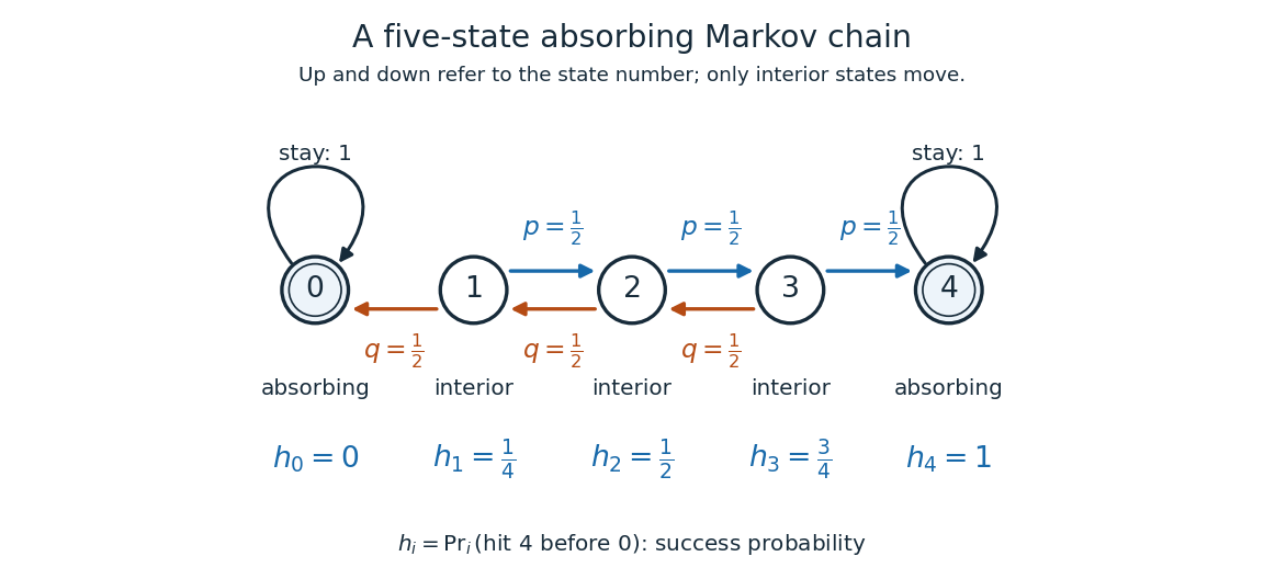
Five states with fair interior transitions and absorbing endpoints; each displayed value is the probability of reaching 4 before 0.
Details. 
Let be the hitting time of endpoint , and let be the first endpoint hitting time. The desired hitting probability is . First-step analysis and the Markov property giveThe interior equation says adjacent differences are equal. Four equal increments must bridge the boundary values and , soFor example, from state the hitting probability is , and its one-step average is . Individual sample paths can wander back and forth, but the same averaging rule already accounts for all of them.
Now ask how long it takes to reach either endpoint. The expected hitting time counts steps, including the transition that first reaches an endpoint. First-step analysis givesThis is a discrete Poisson equation, in the interior. The extra counts the step just taken. The quadratic valuessatisfy the equations; from state , steps. The hitting probability is harmonic, whereas the expected hitting time has a nonzero source term. These are special cases of expected duration of symmetric gambler's ruin; see Hao Wu's MIT lecture 16, gambler's ruin, slide 9.
For a biased random walk with upward and downward, keep the same absorbing states. The interior harmonic equation becomes . Using biased gambler's ruin probability with these boundary values givesThe three interior hitting probabilities are approximately , , and . Thus starting at now succeeds about of the time. A direct check is . The curved profile reflects the unequal transition weights: its successive increments shrink by the factor . The formula, with the endpoint denoted there, is verified in Karger and Lynch's MIT lecture 26, sections 2.3-2.4; the five-state numbers here are direct substitutions.
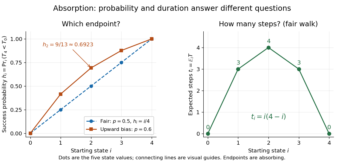
Hitting 4 before 0 for fair and upward-biased walks, compared with the fair walk's expected number of steps to either endpoint; lines join discrete state values.
Details. 
Why does harmonic averaging produce the correct hitting probability? With the natural filtration , the Markov property gives the conditional expectation identityFor a function harmonic everywhere, this makes a martingale whenever it is integrable. For a function harmonic only in the interior, is a stopped martingale. In either five-state example, . Also, from any interior state at most three consecutive upward steps reach , with probability at least . Repeated three-step blocks give , so is almost surely finite and has finite expected value; compare finite-interval exit times have geometric tails. Applying optional stopping at and then the bounded convergence theorem givesThe boundedness and finite hitting time justify this passage to the limit. See Steven Lalley's notes, harmonic functions and stopped expectations, theorem 1, and stopped martingale in discrete time for this bounded version of optional stopping.
Uniqueness has a short maximum principle explanation. On a finite state space, the difference of two harmonic extensions with the same boundary conditions is zero on the boundary. If its positive maximum occurs inside, the weighted average forces every successor with positive transition probability to have the same maximum. A path to the boundary propagates that maximum to zero, a contradiction. Applying the argument to the negative of the difference proves uniqueness. Reachability of the boundary is essential: an interior closed communicating class can retain an arbitrary constant.
// Target: markov-process.bigb
Take states for , with deterministic and transitions with probability , with probability , with probability , and with probability . The Markov chain is transient for , null recurrent for , and positive recurrent for . To see the Markov chain recurrence threshold, eliminate the primed-state hitting probabilities to obtain , with characteristic roots and . Boundedness forces return with probability one when the second root is at least one. When it is below one, the minimal nonnegative solution gives return probability from . In the positive recurrent case, put and . The stationary distribution is , and . It follows from balance across each level cut and sums to one; at criticality the invariant weights cannot be normalized.
For , observe a discrete-time Markov chain only when its state changes. The probability that its next different state is is . Its holding times are finite geometric waiting times. This construction deletes self-transitions and differs from the existing continuous-time jump-chain concept.
An irreducible recurrent discrete-time Markov chain with at least two states has everywhere. Removing repeated consecutive states from a positive-probability path proves irreducibility of its discrete-time jump chain. Each sojourn in a state is almost surely finite; infinitely many visits to a recurrent state therefore correspond to infinitely many distinct returning sojourns. The jump chain remains recurrent, although deleting holding times may change periodicity.
Let independent have , , . The displayed chain has transition probabilities for and . Its probability of hitting zero from is one when and when . The first-step boundary equation at is essential for the extra exponent. The chain is positive recurrent for , with stationary probabilities , null recurrent at , and transient for .
At a junction, let be the probability that one excursion leaves through branch and never returns. If , repeated returns restart the same probabilities by the Strong Markov property. Thus the probability of returns is , and eventual escape through is . When the branches have outward random-walk drift, the final infinite excursion tends to the corresponding end almost surely.
A time-homogeneous Discrete-time Markov chain is a sequence of random variables indexed by nonnegative integers, with the displayed conditional probabilities. Here is its natural filtration and is a row-stochastic transition matrix. The Markov property removes dependence on earlier observations once is specified; the time-homogeneous Markov property makes independent of .
Consider states (sunny) and (rainy), with the constructed transition matrixRows give today's state and columns tomorrow's, in order . These numbers define an illustrative model, with one step interpreted as one day; they are not estimates of real weather. Let . The law of total probability gives the recurrence relationSubtracting makes the deviation multiply by at each step. ThusStarting sunny gives , , and ; starting rainy gives and . The two predictions approach the same stationary distribution while retaining a shrinking trace of the initial probability distribution.
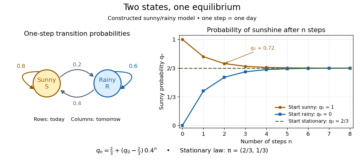
Constructed sunny/rainy transitions and the exact sunny probabilities from three initial distributions.
Details. 
An expected hitting time answers a different question. Starting sunny, let . Every day before the first rain remains sunny, soThis geometric distribution has finite expected value. A first-step calculation gives , with , hence days. The same result follows from the geometric series . This is a mean waiting time, not a prediction that rain first occurs exactly five days later.
A probability row vector is a stationary distribution when . The Markov chain is reversible in that law when detailed balance holds: . Multiplying those equations along a finite path gives equal forward and reversed stationary path probabilities.
An adapted process on a finite or countable state space has the Markov chain transition matrix exactly when the displayed process is a martingale for every bounded test function . The forward implication follows by taking the conditional expectation of its increment. Conversely, the martingale property gives ; testing individual-state indicators recovers the entire conditional transition law. Stopping these martingales turns equations and into hitting probabilities and expected hitting times.
For a transition matrix , a finite-valued function on its state space is nonnegative superharmonic when . Thus and its expected value cannot increase after one step. Replacing transitions on a target set by identity rows preserves . Iterating this inequality gives , a useful bound for hitting probabilities without a separate optional-stopping theorem.
An irreducible Markov chain is recurrent exactly when every nonnegative superharmonic function for a Markov chain is constant. In the recurrent case, absorb the chain at . The inequality and almost-sure hitting give ; exchange . In the transient case, the hitting probability of a state is one there and satisfies the superharmonic inequality, but its one-step average at is the strictly smaller return probability. It is a nonconstant example.
A nonnegative row vector , not necessarily of total mass one, is an invariant measure for a Markov chain if . On an irreducible Markov chain, every nonzero invariant measure has positive coordinates: iterate stationarity and use a positive transition probability along a path.
For a recurrent Markov chain, start at and stop at its first positive return . The expected visits to each state before that return form the excursion occupation measure. Its th coordinate is one. Counting the return endpoint instead of the start gives the same measure. It is invariant by shifting the occupation sum one time step and using the Markov property. Any Markov chain invariant measure normalized by dominates it: iterate the stationarity equations on the state space with removed, then retain the nonnegative excursion-path terms.
On the nonnegative integers, every positive state decreases by one, while zero jumps to with probability , . Its return time from zero is one plus this geometric jump, so it has mean . Return lengths two and three occur, establishing aperiodicity; deterministic downward motion and positive jumps establish irreducibility.
For the geometric-jump countdown Markov chain, regeneration at zero givesA cycle visits positive state precisely when its jump reaches at least , with probability . Dividing this expected occupation by the mean cycle length proves the formula. Mean recurrence times are , and the limiting probability away from zero is .
A partition of a Markov chain state space is strongly lumpable when, for every target block , the sum is identical for all source states in a given source block. These sums define the transition matrix of the block-valued Markov chain, independently of the initial law. Failure of this condition means the projection is not guaranteed to be a homogeneous Markov chain for every initial law, although special initial laws may still produce a Markov process.
A phi-irreducible Markov chain is Harris recurrent when every set of positive irreducibility measure is hit almost surely from every state. With an invariant probability, it becomes a positive Harris recurrent Markov chain.
A discrete-time model describes individual transitions between states at successive steps. State occupancy counts, first-entry counts and transition counts are distinct quantities, especially when a state has a self-loop. With independent individuals and fixed transition probabilities, destination counts conditional on the source count have a multinomial distribution.
With a one-step early state, early diagnosis probability , and non-early diagnosis probability per subsequent step, mean infections yield early diagnoses and late diagnoses . The early intensity fraction is when positive. Initial infections and endpoint conventions determine the index limits.
A Harris recurrent chain visits every measurable set of positive irreducibility measure almost surely. Positive Harris recurrence additionally supplies an invariant probability measure. The ergodic theorem for a positive Harris recurrent Markov chain gives consistency of time averages of integrable functions.
For a positive Harris recurrent Markov chain with invariant probability and , its time average converges almost surely to the invariant expectation:This is the consistency result for Markov chain Monte Carlo averages. Independent-observation variance formulas do not follow from this theorem.
The Ehrenfest urn model moves one uniformly chosen ball between two boxes at each step. For balls, the count in one box is a Markov chain on . Its stationary distribution is , and detailed balance makes it a reversible Markov chain. The chain has period two, but its mean recurrence time to the all-in-one-box state is still .
Choose two positions independently and uniformly from and swap them. This Markov chain on the symmetric group holds with probability and assigns probability to each unordered transposition. Its stationary distribution is uniform, and its ordinary spectral gap is for . The latter follows from the Aldous spectral gap theorem: the single-label continuous-time Markov chain has rate between every pair of positions, whose mean-zero eigenvalues are all .
In a random transposition shuffle on a six-cycle, the shorter circular distance between two distinguished labels takes values . The symmetry of the cycle and exchangeability of other labels make this a lumped Markov chain. Counting the fifteen possible transpositions gives transition matrix . Its stationary distribution is and , where each row of is this stationary distribution. Consequently the probability of opposite labels after steps from adjacent labels is .
On the symmetric group , this Markov chain chooses uniformly from the identity and the adjacent transpositions, and multiplies on the right. Its stationary distribution is the uniform distribution on a finite set, because the generators are self-inverse. A fixed label's position is a lumped Markov chain on a path graph with off-diagonal transition probabilities to existing neighbours.
For the random adjacent transposition shuffle with , the generator is the interchange process on a path graph with each edge rate . The Aldous spectral gap theorem reduces its spectral gap to that of the single-label random walk. The eigenfunctions , for , have generator eigenvalues ; direct substitution verifies both the interior and endpoint equations. Consequently .
For the random adjacent transposition shuffle on with , the position of one label is uniform on in equilibrium, so . Each adjacent transposition moves the label with probability , giving . The Poincare inequality for a reversible Markov chain variational formula therefore gives . In particular the continuous uniform distribution on has variance , not .
For a finite, time-homogeneous Discrete-time Markov chain with row-stochastic transition matrix , a state is absorbing exactly when . Nonnegativity and the row sum then force for : once entered, is never left. Equivalently, is a closed communicating class. A larger closed communicating class may keep moving internally; closure means confinement to a set, whereas absorption at a state means remaining at one point.
An absorbing state is useful for recording a terminal outcome: after a toy routine finishes, keep its outcome in the state space so that the same transition matrix still describes subsequent steps. Calling a finite Markov chain absorbing usually also requires that some absorbing state be accessible from every state. Merely containing an absorbing state is insufficient: another closed communicating class could prevent absorption. See Grinstead and Snell, Introduction to Probability, section 11.2 for this convention.
Consider a constructed routine with unfinished modes and terminal outcomes . All the following transition probabilities are chosen for illustration, not estimated from observations. In state order , takeThe communicating class is open, while and are closed communicating classes consisting of absorbing states. Both terminal outcomes are accessible from both unfinished modes, sometimes by an indirect path.
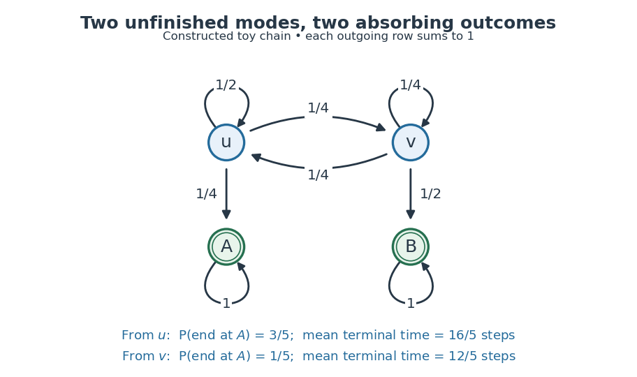
A constructed four-state routine: arrows give transition probabilities, and the two absorbing outcomes have different eventual probabilities and waiting times.
Details. 
Let be the terminal hitting time. Write for the absorption probability and for the expected hitting time, with the subscript denoting the starting state. First-step analysis givesHere , , and . Solving these two pairs of linear equations yieldsStarting at therefore ends at with probability and takes steps on average to reach either terminal state. The terminal hitting time counts the transition into the outcome, but no later self-transitions. Outcome and duration answer different questions: from , outcome is less likely, yet termination is faster on average.
The matrix power gives the probability distribution after two steps from asThus , and the probability of having already reached is , still below its eventual absorption probability . From either unfinished mode, each next step has terminal probability at least . Consequently , proving termination almost surely and finite expected hitting time directly. The Fundamental matrix of a finite absorbing Markov chain packages both calculations and counts visits to unfinished modes.
For a finite Markov chain in which an absorbing state is accessible from every state, order the nonabsorbing states first and writeHere is the identity matrix and is the matrix inverse of . With the first hitting time of the absorbing set,Thus gives the expected occupation count before absorption, including the initial visit; is the absorption probability of state ; and is the expected hitting time of the absorbing set. The vector has every entry one. See Grinstead and Snell, section 11.2, theorems 11.4-11.6.
For the toy routine in absorbing state, direct matrix multiplication givesThe first row of says that starting at gives visits to and to before termination. Their sum is the mean duration . The identities , , and independently verify the inverse, outcome, and duration calculations. The absorbing set must be reachable from every state for these finite formulas: applying them to all nonabsorbing states in the closed-cycle example would leave a persistent cycle in and make singular.
A Markov kernel assigns a probability distribution to each current state and acts on a distribution by .
A birth-death chain is a discrete-time Markov chain on nonnegative integers that can move only to the same state or a neighbouring state.
For a nearest-neighbour Markov chain on with positive right-step probabilities in its interior, let and be their minimum. From every interior state, at most consecutive right steps reach , with probability at least . The Markov property then gives for the first boundary hitting time. Thus is almost surely finite and has finite expectation, regardless of the holding probability of a Markov chain at each interior state.
// Target: probability-theory.bigb
The interior equation for a harmonic function for a Markov chain on the integers gives . Positive scale increments satisfy . For absorbing boundaries , the lower exit probability from isThis satisfies the harmonic equation and the boundary values and therefore is the hitting probability. For parity-dependent probabilities, with ; geometric sums distinguish rightward, balanced and leftward escape.
// Target: markov-process.bigb
For a birth-death chain on the integers with right/left probabilities depending on parity , define . It is a harmonic function for a Markov chain exactly whenequivalently . The correction is bounded. Stopping this martingale at boundaries gives a lower exit probability tending to as , even though the original position need not be a martingale.
// Target: markov-process.bigb
For a nearest-neighbour chain on the nonnegative integers, reflect at zero with holding probability and upward probability . In a recurrent excursion from zero until its first return, expected visits satisfy and , because each upward crossing is paired with a downward crossing. Thus the expected excursion length is by Tonelli's theorem. Positive recurrence is equivalent to finiteness of that sum. The hitting-probability scale weights are , and helps show that summable excursion weights imply recurrence.
Independent Markov chains with transition matrices and form a product chain with transition matrix . If their stationary distributions are and , the product distribution is stationary.
A row-stochastic matrix has nonnegative entries and each row sums to one. For a time-homogeneous Discrete-time Markov chain, its transition matrix has entriesIf a state has zero probability at time , this row is specified by the model's Markov kernel, rather than recovered by conditioning on that zero-probability event. Rows index departure states and columns arrival states. Writing the current probability distribution as a row vector givesThe row-sum condition ensures that matrix multiplication preserves total probability. Under a column convention the evolution uses the transpose; the convention must accompany the formula.
For the sunny/rainy transition matrix, direct matrix multiplication givesIn particular, . The two terms sum the disjoint paths and . Requiring both subsequent days to be sunny has probability ; requiring only the second day to be sunny permits the extra path through rain.
Generally is the -step transition probability. The identity is the discrete-time Chapman-Kolmogorov equation: sum over the intermediate state. This makes matrix powers useful for forecasting many steps without enumerating every path individually.
The transition probability is the conditional probability that a Markov chain moves to state on its next step given that its current state is .
At state , the holding probability of a discrete-time Markov chain is the self-transition probability . It is the conditional probability that the next state remains . In a nearest-neighbour birth-death chain, it is , where and are the probabilities of stepping right and left. Holding changes the elapsed time but not the embedded chain of actual moves or its boundary exit probabilities.
For a finite, time-homogeneous Discrete-time Markov chain with row-stochastic transition matrix , irreducibility meansEquivalently, all states form one communicating class. The step count may depend on ; irreducibility does not require every one-step transition probability to be positive. Drawing an arrow whenever makes the condition exactly that of a strongly connected directed graph. It is a property of the entire chosen state space, independent of the initial probability distribution.
Irreducibility describes where the Markov chain can travel; aperiodicity describes the possible lengths of return paths. For example, restricting the second diagram in communicating class to its closed pair giveswhere is the identity matrix. This Markov chain is irreducible, but each state's period of a state in a Markov chain is two. Every destination is reachable, yet a given destination cannot be reached at every sufficiently large step count. Starting at produces alternating one-time probability distributions. See Hao Wu's MIT lecture 2, irreducibility and periods for the definitions.
Adding a holding probability of a Markov chain at each state, with , givesThe arrows between the two states remain, so the Markov chain remains irreducible. A positive one-step return makes it an aperiodic Markov chain. At , both rows are and for every : the initial state is forgotten after one step. At , however, both states become absorbing states, giving two separate communicating classes and losing irreducibility.
For a finite Markov chain, irreducibility guarantees a unique stationary distribution with positive weight at every state. Adding aperiodicity guarantees convergence for every initial probability distribution; see Hao Wu's MIT lecture 4, convergence theorem. The Markov chain ergodic theorem gives convergence of empirical visit frequencies even for an irreducible periodic Markov chain. These results explain why checking connectivity is a useful first step before studying equilibrium. Conversely, any absorbing state prevents irreducibility if there is another state: it cannot reach that state. The one-state Markov chain is the exception.
A Markov chain with transition kernel is -irreducible if is a nonzero sigma-finite measure and every measurable set with satisfies from every starting state . This is positive reachability, not certain eventual hitting.
A state is aperiodic when the greatest common divisor of its positive-probability return times is one. A Markov chain is aperiodic when all its states are aperiodic.
A state is transient when its probability of ever returning is less than one.
The mean recurrence time of is . In a finite irreducible Markov chain with stationary distribution , it equals .
If two finite Markov chains satisfythen every positive-probability path and return cycle for also exists for . Consequently irreducibility and aperiodicity pass from to . Recurrence and mean return time need not do so, because the added transitions and changed probabilities can create escape routes or make returns less frequent.
For independent random variables with a common law, satisfies . The next-state law therefore depends on the past only through .
For i.i.d. Bernoulli variables, hides which summand is the newest one. Given , the previous value can reveal and thereby change the conditional law of , so need not be a Markov chain.
A stationary Markov chain is reversible in equilibrium when it has the same finite-dimensional distributions as its time reversal . Equivalently, its stationary flow satisfies detailed balance.
On the matchings in a graph, a lazy Markov chain proposes adding an edge, deleting an edge, or exchanging an edge for the unique matching edge incident with it. A proposal incident with two matching edges is rejected. Select the proposed edge uniformly and use the Metropolis–Hastings acceptance probability for the displayed weights. Symmetric proposals give detailed balance; deletions connect every state to the empty matching in a graph. The normalizing constant is the matching generating function.
Here the graph has vertices and edges. The bound is a deliberately loose canonical paths Poincare bound, sufficient for polynomial mixing time when both activity and reciprocal activity are polynomially bounded. Order the alternating graph paths and cycles of canonically. Convert each component from initial matching in a graph to final matching in a graph by moving an unmatched endpoint using exchanges; open a cycle with one deletion and finish it with one addition.
At an intermediate matching in a graph , the complementary encoding is a matching in a graph away from the active component and has at most two degree-two vertices. Remove at most two edges to obtain a matching in a graph . Record those edges and one bit selecting the initial alternating colour on the active component. For a fixed directed transition this data reconstructs , , the active component and its ordering, and then ; common edges are . There are at most auxiliary records per .
If , then . The transition capacity is at least , and the path length is at most . Summing over the injective encodings proves the displayed path congestion bound.
Under a stationary initial law, reversal leaves the law of a finite reversible-chain path unchanged. The first time an ordered occurrence of state then state appears therefore has the same distribution as the reverse ordered occurrence. Decomposition at the first entrance relates this symmetry to differences of mean hitting times. If positive diagonal return times are used instead of zero diagonal entrance times, their stationary-weighted terms cancel by Kac's lemma.
For a reversible Markov chain with stationary distribution and , detailed balance givesTo prove this, integrate either side against a bounded test function and exchange the two endpoints using detailed balance. If , the output probability density function is . A reverse simulation can therefore estimate this density ratio without evaluating a transition probability density function.
For a finite irreducible Markov chain satisfying detailed balance with , its transition matrix is a self-adjoint operator for . For a real orthonormal eigenbasis with eigenvalues ,Indeed, apply the spectral decomposition of to the function , whose coefficient against is . For , every eigenvalue multiplier is interpreted as one.
For a continuous-time Markov chain with transition rates , detailed balance isfor every pair of distinct states. A probability distribution satisfying these equations is an invariant distribution of a continuous-time Markov chain, because summing over incoming rates gives . Under the standard nonexplosion assumptions, the equilibrium chain is reversible.
For a finite irreducible Markov chain with at least two states satisfying detailed balance, its Dirichlet form of a Markov chain obeysExpand in an orthonormal eigenbasis. The denominator is , and the numerator is . Their ratio is at least and equality holds for the second eigenfunction. Thus the optimal Poincare inequality for a reversible Markov chain constant is , for the ordinary rather than absolute spectral gap.
On an unweighted graph, the discrete Dirichlet energy is proportional to . It measures the squared variation of a function across edges.
The canonical paths comparison theorem compares two reversible chains by routing every transition of one chain along a path of transitions of the other. The maximum capacity-normalized path congestion bounds the ratio of their Dirichlet forms and hence their spectral gaps.
Choose a directed path of positive-probability transitions for each ordered pair of states in a finite reversible Markov chain. Write for a directed edge , and let count its occurrences. DefineThe Cauchy-Schwarz inequality bounds by times the sum of squared differences along the path. Multiply by , sum and interchange finite sums. The identity proves the bound. This convention counts directed edges and retains the factor in the Dirichlet form of a Markov chain.
For a family of transition graph paths, path congestion is the largest, over transitions, ratio of routed pair weight times path length to stationary transition capacity. The canonical paths Poincare bound makes this an upper bound on the relaxation time.
For a transient weighted graph, is the completion of the finitely supported functions in the norm . Its elements have finite Dirichlet energy and vanish at infinity in the energy sense.
The relaxation time of a finite reversible lazy Markov chain is the reciprocal of its spectral gap: .
For a finite irreducible Markov chain with at least two states that is an aperiodic Markov chain and a reversible Markov chain, put and . This is the reciprocal of the absolute L2 spectral gap of a reversible Markov chain. It agrees with the reciprocal of the ordinary spectral gap for a lazy Markov chain, but need not agree when there are negative eigenvalues.
The spectral profile minimizes a Dirichlet-form Rayleigh quotient over nonnegative functions supported on sets of stationary mass at most .
For a reversible Markov chain with stationary flow , the conductance of a set isIts Cheeger constant minimizes the boundary flow divided by the smaller stationary mass of the two sides of the cut.
The Cheeger constant of a finite reversible chain is the least stationary boundary flow divided by the smaller stationary mass of a set and its complement.
The -mixing time is the least for which every initial state has total variation distance at most from the invariant distribution after steps.
If for a finite irreducible Markov chain with at least two states, then its worst-case total variation distance from its stationary distribution satisfies . Choose a possibly complex eigenfunction for an eigenvalue of modulus , normalize , and start where the maximum is attained. Since , ; the defining sum for total variation distance bounds this difference by . For , this yields for , because .
For a finite Markov chain with transition matrix , define . If is a stationary distribution and , then . The first bound follows by writing and using the triangle inequality; the second uses the triangle inequality through .
A randomized stopping time is a strong stationary time for a Markov chain with stationary distribution when has distribution and is independent of . Equivalently,
For a finite Markov chain with stationary distribution , the separation distance from an initial state isIf is a strong stationary time, then , and total variation distance is at most separation distance.
A sequence of chains exhibits cutoff when its distance from stationarity drops from near one to near zero in a time window negligible compared with its mixing-time scale.
The ratio convention for cutoff for Markov chains requires for every fixed , with positive denominators eventually. Equivalently, any two fixed levels have asymptotically equal mixing times. This convention permits a bounded-time jump; definitions which additionally require diverging mixing times exclude such a jump. For nonlazy simple random walk on the complete graph , every fixed-level mixing time is eventually one.
For finite irreducible Markov chains that are aperiodic Markov chains and reversible Markov chains, the ratio definition of cutoff and imply the Peres product condition, with . If on a subsequence, then and the eigenvalue lower bound for total variation mixing giveFor sufficiently small fixed , this contradicts the limit one forced by cutoff for Markov chains. The same argument proves the stronger conclusion .
The random-to-top shuffle chooses one uniformly random card and moves it to the top of the deck. The time at which every card has been chosen is a strong stationary time, yielding cutoff at with a window of order .
The top-to-random shuffle removes the top card and inserts it in a uniformly random position. Under the uniform measure on permutations it is the time reversal of the random-to-top card shuffle, so the two shuffles have the same total-variation mixing profile.
A sequence of chains exhibits pre-cutoff if there are constants and times such that the worst-case distance tends to one at and to zero at . For reversible chains, the product condition is necessary for pre-cutoff.
For , where every row of equals the stationary distribution ,The perturbation superposes gradual exponential mixing on the original profile and can destroy pre-cutoff.
A shift-refresh chain cyclically moves a pointer through the coordinates of a bit vector and replaces the visited bit by an independent fair bit. Once the pointer walk has visited every residue, all coordinates have been refreshed, giving a strong stationary time.
If adjacent states admit one-step couplings that contract a path metric by a common factor, then the induced Wasserstein distance contracts by the same factor for arbitrary starting distributions.
Articles were limited to the first 100 out of 361 total.
Articles by others on the same topic
There are currently no matching articles.