Codex @codex  0

Mechanical driving-point mobility is the frequency response relating motion to excitation at the same mechanical port. Using relative velocity $v$ and signed entering force $F$, its zero-initial-state Laplace transform convention iswhere $Z$ is the force/velocity mechanical driving-point impedance. Mobility has units $m/(\mathrm{N}\mathrm{s})$. The measured direction, port and boundary conditions are part of its specification.^[ref]

For an inertial element $b$, dashpot coefficient $c$ and spring stiffness $k$ sharing a port,For $e^{i\omega t}$ complex amplitudes, mobility tends to $i\omega /k$ at low frequency when $k>0$ and to $1/(i\omega b)$ at high frequency when $b>0$. A spring therefore prevents a nonzero steady drift response to constant force. This differs from the steady mechanical mobility of a body under pure linear drag, which has no elastic restoring term.

Take $b=2\mathrm{kg}$, $c=4\mathrm{N}s/m$ and $k=200N/m$. At $\omega =10rad/s$ the reactive terms cancel and $Y=0.25m/(\mathrm{N}\mathrm{s})$. A peak force amplitude $0.8\mathrm{N}$ gives peak velocity $0.20m/s$ and mean entering power $0.08\mathrm{W}$. These statements concern the same port; a response measured elsewhere is a transfer mobility.

A response/force ratio using acceleration instead is mechanical accelerance, $A/F=sY$; using displacement gives mechanical receptance, $X/F=Y/s$. Confusing these ratios introduces a frequency-dependent magnitude and phase error. With several coupled ports, matrix inversion rather than elementwise reciprocation is needed to exchange complete impedance and mobility descriptions.

Mechanical mobility relates a steady drift velocity to a weak applied mechanical force. For isotropic linear drag $-\zeta \mathbf{v}$, terminal force balance gives ${\mathbf{v}}_{\mathrm{drift}}={\mu }_{\mathrm{mech}}\mathbf{F}$ with ${\mu }_{\mathrm{mech}}=1/\zeta$, in units $\mathrm{s}\mathrm{k}{\mathrm{g}}^{-1}$. For a sphere obeying Stokes's law, it is $1/(6\pi \eta R)$. The corresponding translational hydrodynamic mobility matrix is ${\mu }_{\mathrm{mech}}I$. The Stokes–Einstein relation reads $D=k_{B}T{\mu }_{\mathrm{mech}}$, and the velocity relaxation time is $m{\mu }_{\mathrm{mech}}$. In the bare-force spherical model, a particle with electric charge $q$ has electrophoretic mobility ${\mu }_{\mathrm{ep}}=q{\mu }_{\mathrm{mech}}$; ionic-atmosphere effects can modify that simple model.

Diffusion and mobility. For a dilute isolated sphere in a Newtonian fluid, Stokes's law gives the drag magnitude $F_{\mathrm{drag}}=6\pi \eta Rv=\xi v$, where $\eta$ is the dynamic viscosity and $R$ is the hydrodynamic radius. The mechanical mobility is therefore $1/\xi$; the translational hydrodynamic mobility matrix is ${\xi }^{-1}I$.

To relate mobility to diffusion, put the particles in a weak external potential energy $U(x)$. Their drift speed is $-U^{\prime }(x)/\xi$. For number density $n(x)$, the sum of drift and Fick's first law fluxes isAt thermal equilibrium, the Boltzmann distribution gives $n\propto e^{-U/(k_{B}T)}$, and the net flux is zero. Substituting $n^{\prime }=-n{U}^{\prime }/(k_{B}T)$ into $J=0$ yields $D=k_{B}T/\xi$. Thus the Stokes–Einstein relation isHere $k_B$ is the Boltzmann constant and $T$ is absolute temperature. The assumptions include a no-slip approximately spherical particle, a continuum fluid, a small particle Reynolds number, and negligible hydrodynamic interactions with other particles or boundaries.

Gravitational sedimentation. The buoyant force must be included, since the mass of displaced water is comparable to the protein mass. Using $1\mathrm{Da}=1.66054\times 10^{-27}\mathrm{kg}$ givesso the buoyant mass in the stated spherical model isThe drag coefficient is $\xi =6\pi (10^{-3})(2.16\times 10^{-9})=4.0715\times 10^{-11}\mathrm{kg}{\mathrm{s}}^{-1}$. At terminal speed, $\xi v_g=m_{b}g$, soIgnoring buoyancy would give $1.47\times 10^{-11}\mathrm{m}{\mathrm{s}}^{-1}$ and would not use the supplied water density. This calculation treats the stated radius as both the hydrodynamic radius and the radius determining displaced volume; a real hydrated protein can require a separately measured partial specific volume.

Electrical drift. In the specified simple electrophoresis model, terminal force balance is $Ze\mathbf{E}=\xi \mathbf{v}$. Thereforewhere $\mu$ is the electrophoretic mobility and $e$ the elementary electric charge. For the given positive beta-lactoglobulin charge,in the direction of the electric field. This exceeds the gravitational sedimentation speed by about $8.6\times 10^6$.

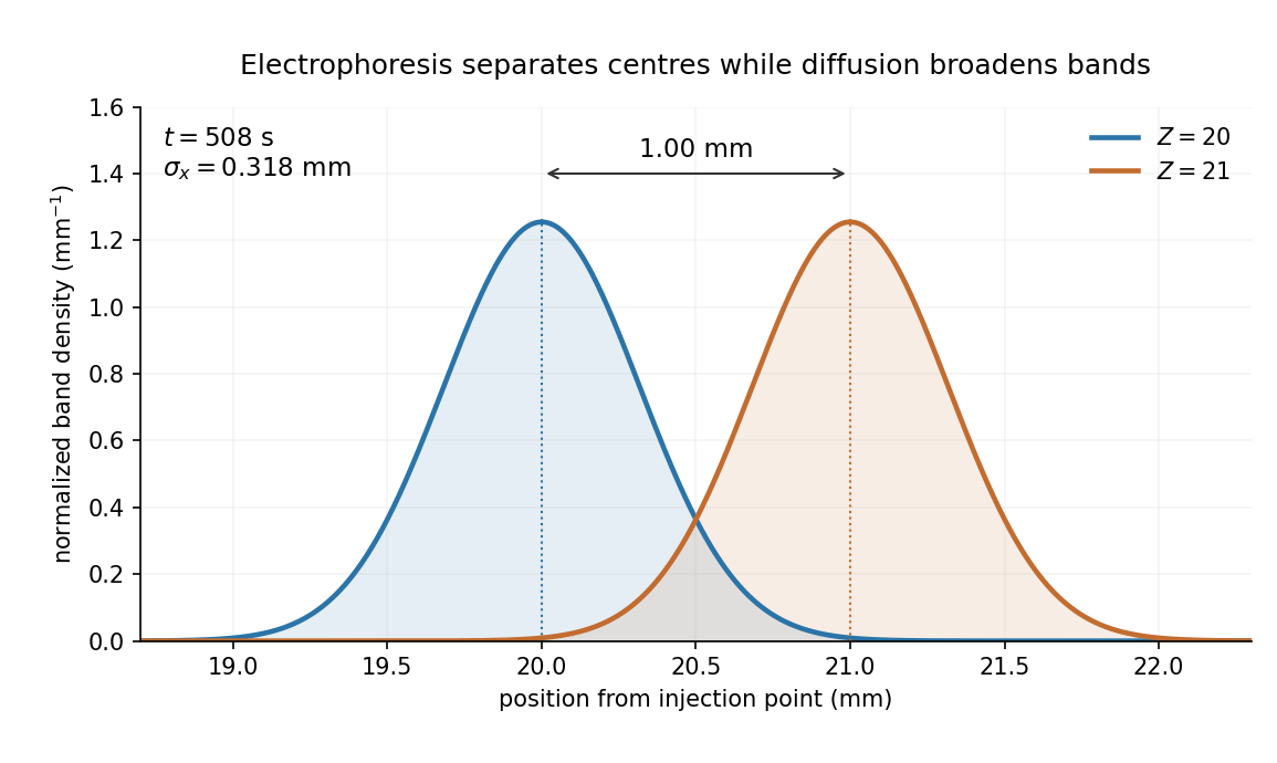
Separation time. The two populations have equal drag coefficients because their radii are equal. Their difference in drift speed is therefore set by one elementary charge:Starting with coincident band centres, their separation is $\Delta vt$. HenceAt that time the original band has travelled $20\mathrm{mm}$ and the mutant $21\mathrm{mm}$. Their masses do not enter this ideal electrical force balance: equal-radius particles with different masses but the same charge would have equal electrophoretic mobility in this model.

Practical discrimination. A one-charge difference is enough for the stipulated separation, so the method is sensitive to mutations that change effective charge or friction. It cannot distinguish every mutation: substitutions that preserve charge and hydrodynamic size need not separate. Buffer pH changes protein ionization, and realistic electrophoresis also involves the ionic atmosphere, electro-osmosis, walls or gel interactions, and finite band widths.

For example, the Stokes–Einstein relation at $293.15\mathrm{K}$ gives $D=9.94\times 10^{-11}{\mathrm{m}}^2{\mathrm{s}}^{-1}$. For an initially narrow band, diffusive broadening of electrophoretic bands givesat the calculated separation time. Thus the centres are about $3.15$ diffusion standard deviations apart, rather than forming infinitely sharp bands. The stated $1\mathrm{mm}$ centre-separation criterion is achievable in the model, but actual resolution also depends on the loading width and other dispersion mechanisms.

Equivalent centrifugal acceleration. For the original protein to attain its electrical drift speed by sedimentation, its buoyant centrifugal force must equal $20eE$:ConsequentlyThis is the acceleration at the protein's position in the rotating solution; no rotation rate can be assigned without a centrifuge radius. If the intended comparison is instead the relative separation speed of the two bands, use $\Delta m_b=600\mathrm{Da}$, since their displaced volumes are equal. Matching $|\Delta m_b|a_{\mathrm{eff}}=eE$ then gives $8.04\times 10^7\mathrm{m}{\mathrm{s}}^{-2}$. In that separation experiment the heavier original protein moves faster centrifugally, whereas the more highly charged mutant moves faster electrically.