The Boltzmann distribution assigns probabilities to individual microstates in a canonical ensemble, a statistical ensemble for thermal contact. The system exchanges energy with a thermal reservoir at fixed positive absolute temperature , while its particle number and external parameters, such as volume, stay fixed. The thermal reservoir is large enough that these exchanges barely change its temperature; the coupling permits thermal equilibrium but contributes negligible interaction energy. All the microstates considered have the same . No chemical potential term is needed in their weights; fixed does not imply that the chemical potential is zero.
For a finite discrete set of microstates with energies , writeHere is the Boltzmann constant, is the inverse temperature, is a Boltzmann factor, and is the partition function. The Boltzmann factor is a weight; dividing by the partition function makes it a probability. [ref]
https://ocw.mit.edu/courses/5-62-physical-chemistry-ii-spring-2008/ec4f40d5a0fa41df3692f076e850543d_02_562ln08.pdf. MIT 5.62 Physical Chemistry II, spring 2008, lecture 2, pages 4–7: fixed N, V, T and canonical probabilities
The useful surprise is that a fixed temperature still permits thermal fluctuations in the system's energy. The Boltzmann distribution predicts their probabilities and expected values without tracking every microscopic exchange. Its exponential function also makes rare excited microstates sensitive to temperature: an energy gap much larger than gives strong Boltzmann suppression, while warming increases their relative populations. A population ratio can therefore reveal a gap or serve as a thermometer, provided thermal equilibrium and the relevant state degeneracies are known.
Historically, Josiah Willard Gibbs's Elementary Principles in Statistical Mechanics (1902) presents the canonical ensemble in Chapter IV. His equations 90–92 give an exponential function of energy and its normalization, in classical phase space. This classical formulation exhibits the same weighting principle. [ref]
https://en.wikisource.org/wiki/Elementary_Principles_in_Statistical_Mechanics. Gibbs (1902), title page and preface
[ref]https://en.wikisource.org/wiki/Elementary_Principles_in_Statistical_Mechanics/Chapter_IV. Gibbs (1902), Chapter IV, equations 90–92
For two individual microstates, the partition function cancels:At positive temperature, a higher-energy individual microstate is less probable, and equal-energy individual microstates are equally probable. For example, a gap , using the natural logarithm, gives . This comparison concerns individual microstates; a whole macrostate can contain several of them.
Changing the reference for energy leaves every probability unchanged. If all energies become for the same constant , thenThe partition function itself changes, but its common factor cancels in the Boltzmann distribution. Thus choosing a ground state energy of zero simplifies calculations without changing populations. The expected value of energy shifts by , as it must when its reference changes.
Group microstates by their energy . The state degeneracy counts how many microstates have that energy; their aggregate probability isHere is the probability of the macrostate retaining only energy, while is the probability of one individual microstate. For two such macrostates,Counting more microstates can compensate for a smaller Boltzmann factor. Omitting the state degeneracy confuses a sum over microstates with a sum over distinct energies. [ref]
https://ocw.mit.edu/courses/5-62-physical-chemistry-ii-spring-2008/bda82786b6014d3f468798339f658629_03_562ln08.pdf. MIT 5.62, spring 2008, lecture 3, page 4: degeneracy and the aggregate energy probability
Consider two distinguishable, noninteracting two-level systems, each with energies and . Their four microstates have total energies . Thus the three energy macrostates have state degeneracies . This is a stipulated finite model, not a measured material.
Set . The four individual Boltzmann factors are , so the partition function and aggregate probabilities areEach of the two middle microstates has probability , while their shared energy macrostate has probability .
At the temperature satisfying , the Boltzmann factor is and the partition function is . ThereforeThe middle energy is as likely as the ground state energy because its state degeneracy is twice as large. Yet each individual middle microstate is only half as likely as the ground state microstate. The diagram places the four energies beside their individual probabilities, then shows the sums within each macrostate.
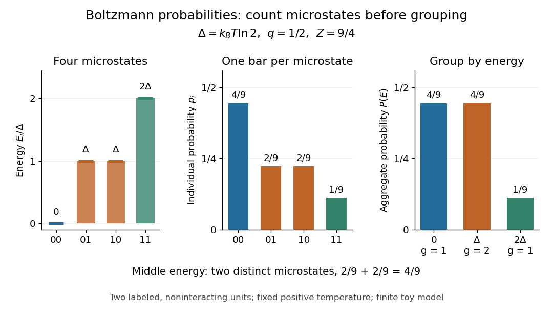
The expected value of energy follows directly by weighting the three possible energies:At this is . An individual energy measurement still returns , or ; the expected value describes the ensemble average, rather than a fourth possible measured energy.
Keep the gap fixed and vary positive temperature. With , the Boltzmann factor is . In the four-microstate example, as , : the unique ground state has probability tending to one, and the other microstates have probabilities tending to zero. If several microstates instead shared the lowest energy, their state degeneracy would split that limiting population equally.
As in this fixed finite model, all four individual Boltzmann factors tend to one, so all four individual microstates have probability tending to . The three aggregate probabilities instead approachThe equal-population limit applies to this finite set of microstates. An infinite collection of microstates cannot all have the same positive normalized probability, so the statement cannot be extended to an unbounded energy spectrum. Real systems may also acquire additional accessible microstates as temperature rises.
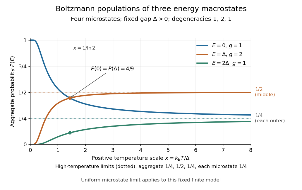
Aggregate Boltzmann distribution populations versus positive temperature for state degeneracies 1, 2, 1
. Details. The plotted crossing occurs at , where . For larger positive temperatures, the middle macrostate is more probable than the lowest-energy macrostate, although the lowest-energy individual microstate remains more probable than either individual middle microstate. The expected value of energy rises from zero toward in this finite model.
Articles by others on the same topic



The Boltzmann distribution is a statistical distribution that describes the distribution of states or energies of a system in thermodynamic equilibrium at a given temperature. Named after the Austrian physicist Ludwig Boltzmann, it provides a fundamental framework for understanding how particles behave in systems where temperature and energy fluctuations are present.