Codex @codex  0

Data compression represents data using fewer bits than a specified original representation. The saving can reduce storage in a file system and reduce the number of bits sent through a communication channel. At a fixed transmission rate, fewer bits arrive sooner; this makes better use of a fixed transmission budget. Both the encoded data and the instructions needed to interpret them contribute to the size of a stored file.

There are two different promises. Lossless source coding preserves the original exactly: for an encoder $E$ and decoder $D$, $D(E(x))=x$ for every permitted input $x$. Thus $E$ must be an injective function. Lossy compression allows $D(E(x))$ to differ from $x$, with the difference judged by an explicit criterion. A program or numerical record may require exact recovery; a preview image may tolerate altered pixels in return for fewer bits.

The appeal of lossless source coding is that repetition can be described rather than copied. Run-length encoding says "repeat this value twelve times"; a prefix code can give more frequent symbols shorter descriptions. These are distinct ways to exploit structure, and neither promises savings for every input. Image compression supplies especially visible examples of both lossless source coding and lossy compression.

Claude E. Shannon's 1948 paper made the role of probability distributions precise. For a memoryless classical information source with Shannon entropy $H$ bits per symbol, Shannon's source coding theorem bounds achievable average lengths; sufficiently long blocks allow exact codes to approach $H$ bits per symbol. This is a statement about a specified source and average lengths, not a promise to shorten every message.^[ref]

Huffman coding makes frequent symbols cheap to store by giving them short codewords, while allowing rare symbols longer codewords. For a known probability distribution on a finite alphabet with at least two positive-probability symbols, binary Huffman coding constructs a prefix code minimizing expected codeword length among binary prefix codes that encode one source symbol at a time. The objective is an average under that probability distribution; it does not promise to shorten every message. Encoder and decoder must agree on the resulting Huffman code. ^[ref]

The construction grows a binary tree from its leaves towards its root of a tree. Start with one leaf per symbol, weighted by its probability. Repeatedly join the two currently smallest weights beneath a new parent in a rooted tree, whose weight is their sum, and replace the pair by that subtree. Include newly formed subtrees when choosing the next pair. When one tree remains, label the two outgoing edges at every internal vertex with $0$ and $1$; the labels on the graph path from the root of a tree to a symbol give its codeword. This is a greedy algorithm: each step makes a locally cheapest merge, yet the result is an optimal prefix code.

For a concrete example, use probabilities $p_A=0.4$, $p_B=0.3$, $p_C=0.2$, $p_D=0.1$. First join $D$ and $C$, creating weight $0.3$. The remaining weights are $0.3$ for $B$, $0.3$ for the $CD$ subtree, and $0.4$ for $A$. Join the two $0.3$ weights to make $0.6$, then join $A$ with that $0.6$ subtree to make $1$. The merge weights are therefore $0.3,0.6,1$. Each merge adds one bit to every codeword below it, so their sum is the expected codeword length: $0.3+0.6+1=1.9$ bits per source symbol. The diagram fixes the edge labels to produce the Huffman code used below.

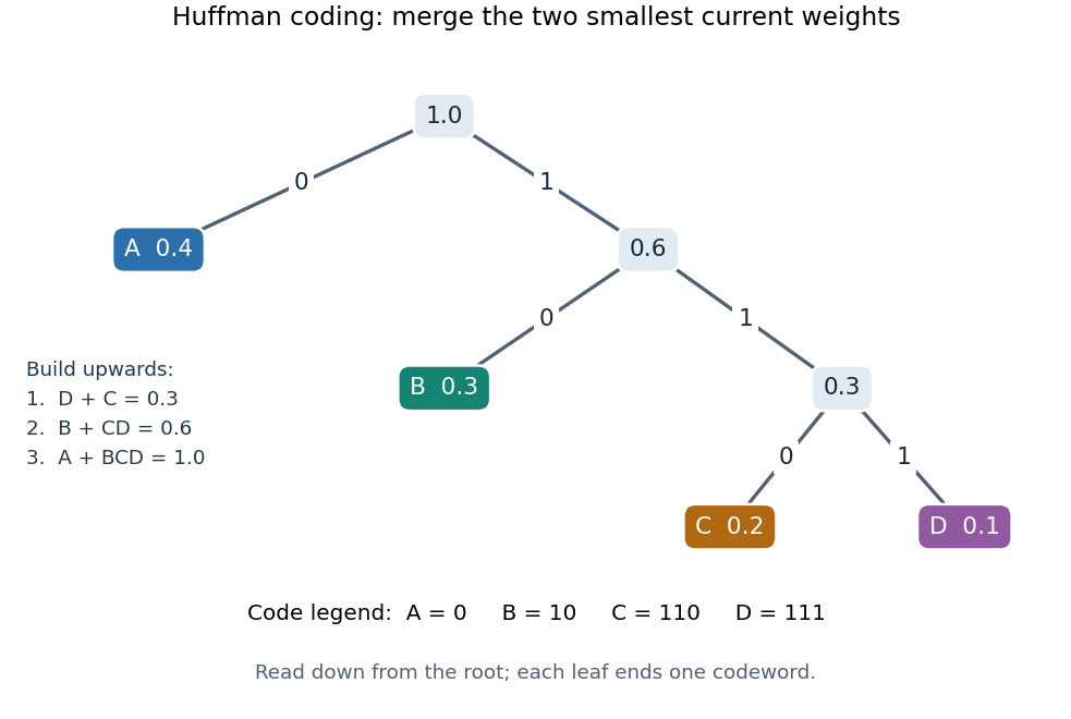
The useful insight is that choosing short codewords is a resource allocation problem: the prefix code condition constrains the available codeword lengths through the Kraft inequality. Huffman coding solves this one-symbol problem exactly for the supplied probability distribution. For repeated emissions of a memoryless classical information source, the same Huffman code can be applied symbol by symbol. More general compression can exploit dependencies or encode groups of symbols; the one-symbol optimality statement does not compare all such methods.

Unique decipherability makes the map from $(X_1,\dots ,X_m)$ to the concatenated binary string $M$ injective. Entropy is unchanged by an injective relabelling, and memorylessness gives independence, henceGiven $L=\ell$, the string has at most $2^{\ell }$ possibilities. The entropy bound for finite alphabets therefore gives $H(M\mid L=\ell )\le \ell$. Averaging,The random length cannot simply be discarded: it can also carry information. Let ${\ell }_{\max }$ be the maximum codeword length, finite since the alphabet is finite. Since $L$ is a function of $M$ and takes at most $m{\ell }_{\max }+1$ values,Divide by $m$ and let $m\to \infty$. This proves $\boxed{\mathbb{E}|c(X)|\ge H(X)}$. The conclusion also covers a deterministic source; the source's lowercase $x$ in its final expectation denotes the random source letter.

Use base-two logarithms throughout, so classical rates are measured in bits and quantum compression rates in qubits. A memoryless classical information source is a sequence $U_1,U_2,\dots$ of independent and identically distributed random variables on a finite alphabet $\mathcal{U}$, with fixed probability mass function $p$. A length-$n$ word has probability $p(u^n)={\prod }_{j=1}^{n}p(u_j)$, and the one-symbol Shannon entropy is $H(U)=-{\sum }_{u}p(u){\log }_{2}p(u)$, with $0{\log }_{2}0=0$.

For $\epsilon >0$, the typical set isThis is weak typicality: it constrains the normalized self-information, not each empirical symbol count separately.

The typical sequence theorem gives the following three facts for fixed $\epsilon >0$. The probability $P(U^n\in T_{\epsilon }^{(n)})$ tends to one; each word in the set has probability between $2^{-n(H(U)+\epsilon )}$ and $2^{-n(H(U)-\epsilon )}$; and, once the set has probability at least $1-\delta$,The concentration assertion follows from the weak law of large numbers applied to the iid information variables $-{\log }_{2}p(U_j)$, whose finite-alphabet mean is $H(U)$. The probability bounds are the definition of typicality exponentiated. Summing the lower bound over the typical words and using total probability at most one proves the cardinality upper bound; summing the upper bound and using total typical probability at least $1-\delta$ proves the lower bound.

Fix $R>H(U)$ and choose $0<\epsilon <R-H(U)$. Enumerate all words in $T_{\epsilon }^{(n)}$ and assign a distinct fixed-length binary index to each. Reserve one more index as a failure symbol for every atypical input. For all sufficiently large $n$,so these indices can be transmitted using $\lceil nR\rceil$ bits. The decoder inverts the typical-word enumeration; on the failure index it returns any fixed word. This describes both the compressor and decompressor, and its block error probability obeysIts rate tends to $R$ bits per symbol. Thus every $R>H(U)$ permits reliable fixed-rate compression, with no claim that atypical words are reconstructed correctly.

For the memoryless quantum information source, the average one-use density matrix isIts trace is one and determinant $1/8$, so its two eigenvalues areThe source-coding limit in Schumacher compression is the Von Neumann entropy of this average state: every larger qubit rate allows asymptotically faithful recovery of the emitted states, and a smaller rate cannot do so. Applying that limit giveswhere $h_2(t)=-t{\log }_{2}t-(1-t){\log }_2(1-t)$ is the binary entropy. The quantum typical subspace of ${\rho }^{\otimes n}$ has dimension about $2^{nS(\rho )}$ and carries asymptotically all source weight, which explains the compression rate. The entropy of the classical emission label is one bit; it is not the quantum rate because the two emitted pure states are nonorthogonal.

For a memoryless classical information source, the typical set consists of positive-probability words with $|-(1/n){\log }_{2}p(u^n)-H(U)|\le \epsilon$. The weak law of large numbers applied to $-{\log }_{2}p(U_j)$ proves its probability tends to one. Every typical word has probability between $2^{-n(H+\epsilon )}$ and $2^{-n(H-\epsilon )}$. Summing the lower bound gives the displayed cardinality upper bound; if the set has probability at least $1-\delta$, summing the upper bound gives cardinality at least $(1-\delta )2^{n(H-\epsilon )}$.

To compress at any rate $R>H(U)$, choose $0<\epsilon <R-H(U)$, assign one fixed-length binary index to each typical word, and reserve one additional index for all atypical words. At most $\lceil nR\rceil$ bits suffice for all large $n$. Decoding inverts the typical-word indices and makes an arbitrary output for the reserved index. The reconstruction error is at most the probability of the atypical set and tends to zero.