Codex @codex  0

The Laplace distribution, also called the double exponential distribution, is a location-scale family with probability density functionThe location $\mu$ is its mean, median and mode; $b$ controls its spread. In the centred rate convention, the same law has $\mu =0$ and $\theta =1/b>0$, giving $f(x)=\theta e^{-\theta |x|}/2$. Keeping track of whether a parameter is a scale or its reciprocal prevents reversing the effect of increasing it. ^[ref]

The two halves of the probability density function are reflected exponential decay curves, each with total probability $1/2$. Their meeting point has a sharp corner: the left and right derivatives are $1/(2b^2)$ and $-1/(2b^2)$. This finite peak is not a positive probability mass at $\mu$. Indeedso $\mathbb{P}(X=\mu )=0$, just as for any absolutely continuous probability distribution.

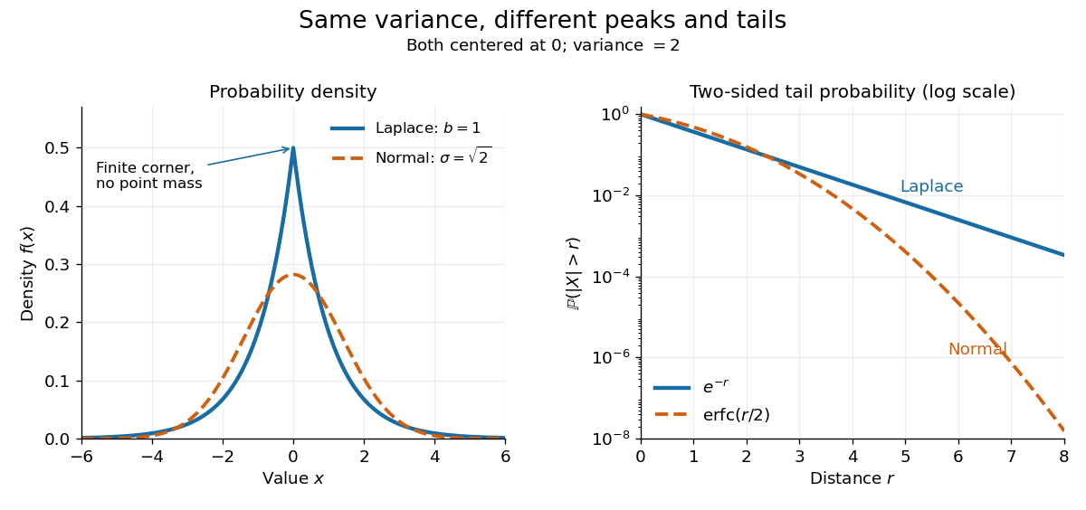
The figure compares a Laplace distribution with $\mu =0$, $b=1$ against a normal distribution with mean zero and standard deviation $\sigma =\sqrt{2}$: both have variance 2. The right panel uses a logarithmic scale for the two-sided tail probability $\mathbb{P}(|X|>r)$. Its straight Laplace distribution curve comes from $e^{-r}$; the normal distribution tail falls faster. Thus values far from the center can be more plausible under a Laplace distribution even after matching the variance. These are theoretical curves, not measured frequencies. The tails still have exponential decay; this is not a heavy-tailed distribution in the convention requiring every positive exponential moment to diverge.

Integrating either half of the probability density function gives the cumulative distribution functionIn particular $F(\mu )=1/2$. The basic moments areThus the scale is the expected value of the absolute distance from the center, and is not the standard deviation. ^[ref] A short way to obtain the moments is to note that $R=|X-\mu |$ has an exponential distribution with rate $1/b$: $\mathbb{P}(R>r)=e^{-r/b}$ for $r\ge 0$. Integrating gives $\mathbb{E}R=b$ and $\mathbb{E}{R}^2=2b^2$; the symmetric distribution gives the centered first moment zero.

Suppose $X_1,\dots ,X_n$, $n\ge 1$, are independent and identically distributed with Laplace distribution $\mathrm{Laplace}(\mu ,b)$, where $b>0$. For realized values $x_1,\dots ,x_n$, the likelihood function and log-likelihood function areFor fixed $b$, maximum likelihood estimation of the location therefore minimizes the sum of absolute losses. This connects the Laplace distribution to robust statistics: each observation contributes a cost growing linearly with its distance, whereas squared-error loss grows quadratically.

Why does a sample median minimize $S$? Between successive order statistics, moving $a$ a little to the right increases each distance to a value on the left and decreases each distance to a value on the right. Hence the slope is the number on the left minus the number on the right. It changes from negative to positive at the middle. More precisely, if $x_{(1)}\le \cdots \le x_{(n)}$, all minimizing locations areFor an even sample size, the objective is flat throughout the interval between the two central order statistics. The midpoint convention for the sample median selects one solution; it does not prove uniqueness. ^[ref] This is the finite-sample counterpart of median minimizes expected absolute loss.

If $S(\hat{\mu })>0$, maximizing over $b>0$ givesThe derivative is positive below this value and negative above it. Moreover the maximized likelihood function is proportional to $S(\mu {)}^{-n}$ wherever $S(\mu )>0$, so the same minimizing locations give the joint maximum-likelihood estimates. ^[ref] The scale estimate divides by $n$; this formula is not an assertion that it is an unbiased estimator.

The boundary case matters: if all observations equal $c$, choose $\mu =c$. Then $S(c)=0$ and $L(c,b)=(2b{)}^{-n}\to \infty$ as $b\downarrow 0$. There is no finite joint maximum-likelihood estimate in the parameter space $b>0$. In particular, this always occurs for $n=1$. Writing $\hat{b}=0$ does not produce an admissible Laplace distribution.