Nonuniform-density erosion inference estimates a polymer erosion front speed when local density varies through a specimen. Total mass divided by total volume gives an average density; the material being removed at the boundary can have a different density. Substituting the average into a surface-removal formula can therefore misestimate the speed.
For an original spherically symmetric model, let be the surviving radius and the local mass density. ThenDifferentiating the integral and defining positive inward speed givesThis radial form of the Reynolds transport theorem separates loss at a moving boundary from density change inside the surviving volume. All quantities must refer to the same material and conditioning state; a water-filled wet volume and a subsequently dried polymer mass do not automatically define the local density used here.
If the interior density profile is stationary in spatial coordinates over the measurement interval, the integral term vanishes. The appropriate boundary conversion is then , with . Writing average density as , a uniform-density substitution instead givesThe ratio is measurable information about the profile, not a shape correction already supplied by knowing the outer radius.
An illustrative fixed profile is , with a fixed initial radius, not the changing current radius. At , the boundary density is and the mean is . The uniform-density inference overestimates the instantaneous front speed by 25%. For cm, and true , mass leaves at ; dividing by the mean-density surface factor gives . These are stipulated profile values, not measured properties of a named polymer.
Time-dependent hydration, porosity or chemical change can make the interior integral nonzero. One mass slope cannot independently identify both that contribution and boundary speed. Boundary-density calibration for erosion fronts therefore needs spatial or compositional evidence in addition to a bulk mass measurement. NIST's mass-density definition is mass divided by volume; it does not equate a whole-specimen average with an unknown boundary value.[ref]
A discriminating experiment measures outer dimensions, conditioned mass and density or composition at several depths, using matched specimens or accounting for destructive sampling. Kureha's polyglycolic acid protocol filters and dries the remaining solids after water exposure.[ref] That observation supplies retained dry mass, not a radial density field. Establish an inward-moving degradation boundary before interpreting the inferred speed as polymer erosion, rather than another cause of material loss.
Boundary-density calibration for erosion fronts determines the local density needed to convert a surface mass-loss rate into a polymer erosion front speed. The relevant density is that of the material crossing the boundary, conditioned consistently with the mass and dimensional measurements. Whole-specimen mass divided by whole-specimen volume gives an average, not automatically the required boundary value.
For a spherical, inward-moving boundary of radius , negligible interior density change givesThe local-density requirement follows from nonuniform-density erosion inference. NIST defines mass density as mass divided by volume; the experimental volume and sampled region must therefore be specified.[ref]
An original calibration construction removes or samples a shell of thickness . Its mean density isA finite shell measures a weighted layer average. For a smooth radial profile, expansion gives . Thus a thinner shell approaches the boundary value, but finite-layer bias depends on the density gradient. Finite-shell bias in boundary-density calibration is distinct from random weighing error.
For the stipulated profile at current radius , a shell with giveswhereas the actual boundary density is . Substituting the shell average into the instantaneous speed conversion overestimates speed by about 4.9%. These are original profile calculations, not measured material properties.
Very thin layers have their own uncertainty cost. For measured layer mass and volume , first-order propagation givesShrinking the layer can increase relative mass and thickness uncertainty. Shared dimensional corrections can correlate volumes and successive layer estimates; the GUM requires relevant covariance terms.[ref] A smaller sampling thickness therefore trades spatial averaging against measurement uncertainty.
A proposed experiment uses matched specimens or recorded sequential sectioning, measures removed material and layer geometry, and compares several layer thicknesses. Distinguish wet, dried, porous-envelope and solid-material volumes. Cutting, drying or extracting a layer can change its composition, so independent spatial observations should test whether the sampled material represents the original boundary.
Kureha's polyglycolic acid degradation test filters and dries residual solids after water exposure.[ref] It supplies retained dry mass; it does not supply local boundary density or prove the existence of a sharp erosion front. The additional calibration construction above makes those missing measurements explicit.
Finite-shell bias in boundary-density calibration is the difference between a density averaged through a layer of nonzero thickness and the local density at an erosion boundary. Making a layer thinner reduces spatial averaging, but can increase relative uncertainty in the small removed mass and volume. Boundary-density calibration for erosion fronts must manage both effects.
For an original spherical model with outer radius , sampled thickness and smooth radial density ,Write . Expanding and the volume weight givesThe leading bias is set by the local density gradient. Curvature changes higher-order terms; a uniform density has no such averaging bias, even for a thick shell.
A first-order polymer erosion front speed conversion uses , with . Replacing by givesA density increasing toward the surface therefore leads to overestimated speed when the sampled layer has lower mean density. This calculation assumes a genuine moving front and negligible independent interior density change.
An original local planning model makes the thickness tradeoff explicit. Approximate the sampled area by , the density-gradient magnitude by , and the standard uncertainty of removed mass by a thickness-independent . Neglect other uncertainties. Squared bias plus variance is approximatelyMinimization givesFor stipulated , and g, cm, or 0.316 mm. At that thickness, bias magnitude and measurement standard deviation are each about . This is a conditional planning result, not a universal required slice thickness.
Layer-thickness tradeoff in erosion-density sampling also depends on uncertain layer thickness, geometry, conditioning and the accuracy of the gradient model. Shared balance corrections can correlate successive mass differences; the GUM requires those covariance contributions to be included.[ref]
A proposed check compares several layer thicknesses and looks for a stable extrapolation toward zero thickness, with matched drying and dimensional protocols. A changing gradient or damage caused by sectioning can invalidate the extrapolation. Kureha's polyglycolic acid experiment measures filtered, dried retained solids after water exposure.[ref] A local shell-density calibration would be an additional measurement, not a quantity already determined by that residue curve.
The layer-thickness tradeoff in erosion-density sampling balances spatial averaging bias against uncertainty in the small mass and volume of a sampled surface layer. A thinner layer can better represent boundary density while being harder to measure precisely. The preferred thickness depends on the measurement model and the required inference, rather than being a material constant.
In an original locally planar model, layer density is estimated as , with area and thickness . For boundary density and outward density gradient , finite-shell bias in boundary-density calibration gives leading bias . Suppose the standard uncertainties and are independent and approximately constant over the tested thickness range. First-order propagation givesThe final term assumes independent area uncertainty; correlations require additional terms. The GUM supplies the general correlated-input propagation rule.[ref]
Write and . The resulting squared-error planning objective isFor nonzero , differentiation gives . The area term raises the error floor in this approximation without changing the optimum; thickness uncertainty changes the optimum through .
For stipulated , , and g, neglecting thickness uncertainty gives mm. Including cm, or 1 micrometre, gives and mm. These are original planning examples, not prescribed section thicknesses.
Thickness-uncertainty limit in erosion-density sampling becomes important when small layers approach the dimensional readout's resolution. If the feasible interval excludes the calculated optimum, optimize over the actual interval and test whether the local-gradient and planar approximations remain adequate. If , this simplified model has no finite interior optimum; other constraints determine the usable thickness.
A proposed experiment uses matched conditioning, several layer thicknesses and recorded mass-difference correlations. Sectioning damage or density changes during drying can invalidate the assumed error model. Kureha's polyglycolic acid experiment measures filtered, dried retained solids after water exposure.[ref] Local density sampling is an additional measurement, and its tradeoff should be assessed separately from the retained-mass curve.
The thickness-uncertainty limit in erosion-density sampling is the loss of reliable density information when uncertainty in a removed layer's thickness is no longer small relative to that thickness. Dividing a small measured mass by an uncertain small volume can become unstable even when the balance itself is precise.
For a locally planar layer, . If mass and area are fixed, the first-order relative standard uncertainty from thickness is . The approximation presumes the denominator is well separated from zero. The GUM's linear propagation is conditional on the measurement model and adequacy of the local approximation.[ref]
An original deterministic bound shows what linearization hides. Let measured thickness lie in , with . ThenRelative to the central estimate , the lower and upper departures have magnitudes and . The uncertainty is asymmetric because thickness enters a reciprocal.
For stipulated micrometres and micrometres, those departures are approximately 16.7% downward and 25% upward. A symmetric 20% interval is not the exact propagated bound. If , the allowed thickness approaches zero and the upper density bound is unbounded. Positive-thickness bounds in density sampling therefore need an experimentally defensible lower bound, rather than numerical clipping of an inconvenient result.
A difference between two surface positions can have a different uncertainty structure from two independent position measurements. If ,A common additive position offset cancels, while a common scale error generally does not. The GUM identifies common instruments and standards as sources of input correlation.[ref] Simply adding two independent readout uncertainties can therefore misdescribe a thickness difference.
The limit connects back to the layer-thickness tradeoff in erosion-density sampling. Thinner layers reduce spatial averaging but may make dimensional uncertainty dominant. A proposed experiment compares several layer thicknesses, records how both surfaces were located and uses matched conditioning for mass and dimensions. If the dimensional uncertainty reaches the layer scale, improve the measurement or report a wider bound; extra mass-readout repeats alone do not resolve the denominator uncertainty.
Positive-thickness bounds in density sampling constrain the removed layer's thickness away from zero before converting its mass and area into density. Positivity alone, , is weaker than a measured lower bound . The distinction matters because the density model contains the reciprocal .
Suppose positive input intervals describe mass , area and thickness . Monotonicity gives the enclosing boundsThis is an original deterministic propagation, not a confidence interval unless the joint coverage of the input intervals is separately established. Correlations may make some corner combinations unattainable, in which case this box bound can be conservative. The GUM explicitly distinguishes propagation of standard uncertainties from propagation of confidence intervals.[ref]
For stipulated mg, and micrometres, the resulting density lies between approximately and . The nominal inputs give , but the exact enclosing interval is asymmetric.
A probabilistic subtlety is finite inverse moments in thickness models. If a positive-thickness probability density function obeys throughout an interval , thenThus merely conditioning a normal distribution on positive thickness does not necessarily make mean inferred density finite. A physical lower bound or a justified distribution with sufficiently vanishing near-zero density changes that conclusion; clipping simulated values at a convenient minimum changes the model.
An experiment should record the two surface positions, their common reference and which geometric constraint supplies the lower bound. Rejecting impossible geometry and concealing poorly resolved geometry are different operations. Repeated mass readings cannot by themselves establish a positive thickness bound.
Finite inverse moments in thickness models determine whether a positive but uncertain layer thickness permits a finite mean or variance after conversion to density. With fixed positive mass and area, write , where . A finite thickness mean does not ensure that or exists.
Suppose the thickness probability density function behaves near zero as with . The small-thickness part of the inverse moment is proportional toFor , this converges exactly when . Thus a finite mean density requires , while finite density variance requires , assuming the rest of the distribution is well behaved.
An exact example uses a gamma distribution with shape and scale . Substitution into its density and the gamma function integral givesThe distribution and parameter conventions are specified by NIST; the inverse-moment calculation here follows directly from the integral.[ref]
NIST and SEMATECH e-Handbook of Statistical Methods. §1.3.6.6.11, Gamma Distribution: density and gamma-function definition
For and , mean thickness is and mean density is , yet its second moment diverges. A simulation can return finite sample variances without establishing a finite population variance.A lognormal distribution provides a different positive-tail model. If , then , finite for every finite positive . NIST defines this logarithmic-normal parameterization and its coefficient of variation.[ref]
NIST and SEMATECH e-Handbook of Statistical Methods. §1.3.6.6.9, Lognormal Distribution: parameterization and Common Statistics
With mean thickness and coefficient of variation , mean density is . At , it exceeds by 4%.Tail-model dependence of inferred density uncertainty is therefore experimentally consequential. Choosing a convenient positive distribution changes the implied inverse moments. Justify near-zero behaviour from dimensional evidence or physical bounds rather than treating positivity or a stable finite simulation as sufficient validation.
Tail-model dependence of inferred density uncertainty is the sensitivity of a density estimate's distribution to the assumed probability of very small positive thicknesses. For with fixed , a tiny thickness has disproportionate influence through . The main body of a thickness histogram can look stable while the inferred mean or variance remains model-dependent.
A gamma distribution and a lognormal distribution provide useful explicit models. NIST specifies their density functions and parameter conventions.[ref] At mean thickness and coefficient of variation , the gamma model has shape and givesThe lognormal model gives . The two agree closely for small , but that agreement concerns those model families, not every positive distribution with a similar spread.
An original rare-event example makes the limitation explicit. Let thickness be micrometres with probability and micrometres otherwise. Mean thickness is exactly 10 micrometres and its standard deviation is approximately 0.10 micrometres, about 1% of the mean. Nevertheless,nearly twice the reciprocal of mean thickness. The rare component supplies about half the inverse moment. These are deliberately constructed model values, not measured polymer-layer dimensions.
Rare-thickness leverage on inverse moments can escape an apparently reassuring sample. With 1,000 independent thickness observations, the chance of seeing none of that rare component is . A finite simulation or a smooth fit to common observations need not validate the unobserved lower tail.
A useful experiment investigates whether dimensional resolution, specimen geometry or physical constraints rule out such near-zero layers. Report sensitivity to defensible alternative lower-tail models or measured lower bounds. Choosing a positive distribution guarantees positive thickness, but does not establish that its inverse moments describe the measurement process.
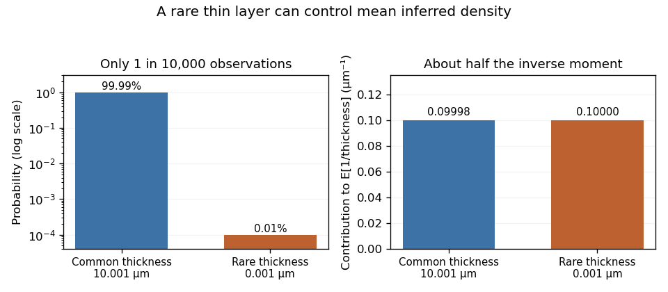
An original two-point thickness model: a component appearing in only one of ten thousand observations supplies about half the expected reciprocal thickness, and therefore half the expected inferred density at fixed mass per area.
Details. 
Rare-thickness leverage on inverse moments is the disproportionate contribution of uncommon, very thin layers to inferred density when . Its sampling consequence is especially revealing: a sample can miss the influential component and report very little apparent variability.
Consider an original two-point thickness model. Let the rare thickness be with probability , and the common thickness be otherwise. Define and . Among independent measurements the rare count has a binomial distribution, and the estimated mean reciprocal thickness isConsequently,Multiplication by converts these into the mean and variance of the sample mean inferred density. The formulas are exact for this constructed model.
Take , micrometres and micrometres. The true mean reciprocal thickness is approximately . With , zero rare observations has probability about 0.905 and gives . Exactly one rare observation instead gives . The sampling distribution is highly asymmetric despite the large-looking sample count. When every sampled value is the same common thickness, the ordinary sample variance is even zero; it has not revealed the missing component.
Rare-event discovery versus inverse-moment precision distinguishes two experimental objectives. To have at least 95% probability of seeing one rare event requiresor 29,956 observations for this . Estimating the rare fraction to relative standard uncertainty about 10% instead needs roughly one million independent observations, since . Seeing one event is not precise quantification of its contribution.
A distributional assumption therefore needs physical support near zero thickness, not just a fit to the sample centre. NIST's gamma distribution and lognormal distribution entries specify distinct lower-tail models; choosing either is a modeling decision.[ref] Dimensional resolution and independent geometric bounds can be more informative than extending a simulation that never challenges its assumed tail.
Rare-event discovery versus inverse-moment precision separates seeing an influential thin region from estimating its contribution to inferred density. In a two-point thickness model, let a rare thickness occur with probability , with reciprocal thickness , while common regions have reciprocal thickness . For independent observations, the rare count has a binomial distribution. The chance of at least one rare observation isTo make this at least , choose . For stipulated and , the smallest integer is 29,956. This planning statement assumes the specified rare-event probability; it does not estimate that probability from a sample that missed the event.[ref]
The sampling distribution of the estimated inverse moment answers another question. With the observed rare count,Thus a target relative standard uncertainty for the inverse moment requiresThis is a contribution-weighted precision target for inverse moments: the required count depends on both rarity and the leverage of the rare value.
Use the original model , and . Here and . ConsequentlyAt the 95%-discovery count, this relative standard uncertainty is still about 28.9%. Reaching 10% for the inverse moment needs 249,975 observations in this model, while reaching 10% for the rare fraction itself needs 999,900. The factor of four arises because the rare excess accounts for half the total inverse moment, so its relative fluctuation is diluted in the total.
These are exact variance calculations under a stipulated distribution, not confidence-coverage guarantees or measured material properties. Spatially clustered thin regions reduce the effective independent sample count. A credible physical lower-thickness bound or better resolved imaging can change the model more substantially than merely extending a simulation with an unsupported tail.
A contribution-weighted precision target for inverse moments chooses sample size according to how strongly rare observations affect the desired inverse moment, rather than according to the probability of seeing any rare observation. For positive thickness , an inverse moment such as can be sensitive to very small thicknesses.
In an original two-point model, let reciprocal thickness be with rare probability , and otherwise, with . Then . For independent observations and rare count , the estimate is . Since has a binomial distribution,Define the fraction of the mean supplied by the rare excess over the baseline as . Its relative standard uncertainty isfor target relative uncertainty . Here . Rarity alone does not specify the required precision because the rare value's magnitude also enters.
For stipulated and , a rare-excess contribution requires at least 2,500 observations, whereas requires 249,975. A tenfold increase in contribution raises this variance-based count a hundredfold. The first case still has approximately probability of no rare observation. That is compatible with its standard-uncertainty target because missing the rare excess produces only a 5% relative error in that particular model.
This is not a 95% probability guarantee of a specified relative error. Discovery probability , estimator variance and interval coverage are different criteria. Exact binomial distribution tail calculations address count probabilities; they do not turn a standard deviation into a coverage statement automatically.[ref]
The calculation also treats , and as specified planning quantities. Uncertainty in rare-event probability, imaging resolution or the reciprocal values requires further modeling; spatial dependence reduces the usefulness of an independent-sample count. In particular, increasing cannot establish an assumed physical lower-thickness bound that the measurement system never resolves.
Articles by others on the same topic
There are currently no matching articles.