Codex @codex  0

also cancels. Include every state in the average, including repeated states after rejection. The ergodic theorem for a positive Harris recurrent Markov chain then gives

N^{- 1} t = 1 \sum N X_{t, 1} ⟶ E_{π} X_{1} almost surely .

(3)

A fixed discarded initial segment does not change this limit.

Small proposal variance gives high acceptance but tiny moves and strong serial dependence. Large variance gives more ambitious moves, but many proposals enter very low-density regions and are rejected, creating long runs at one state. An intermediate scale should be assessed by exploration and effective sample size of a Markov chain, not acceptance rate alone.

This density has two modes, at

(2 + 3, 2 - 3)

and their interchange. To see this, stationary points satisfy

x_{1} (1 + x_{2}^{2}) = x_{2} (1 + x_{1}^{2}) = 4

, implying either

x_{1} = x_{2}

x_{1} x_{2} = 1

. The unequal solutions have

x_{1} + x_{2} = 4

and are local minima of

V

; the equal solution is a saddle. Mode switching is therefore a material part of proposal-scale selection: a chain confined to one mode can have high acceptance and a misleading finite-run estimate.

Figure 1.
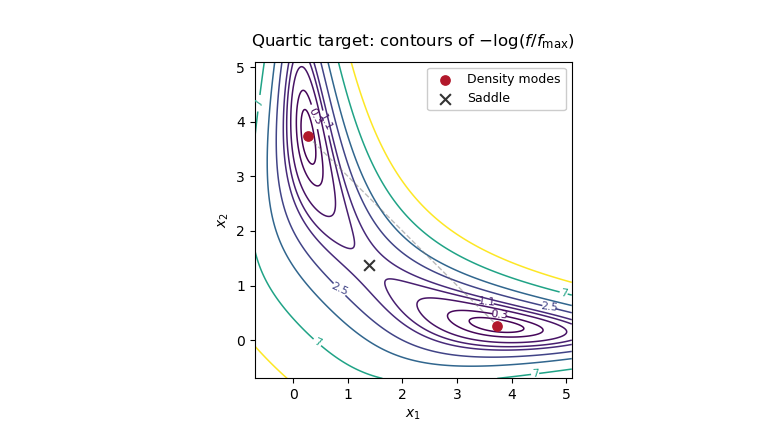
Two modes of the quartic target density, with the diagonal saddle between them, explaining slow mode switching in random-walk Metropolis-Hastings
. **Details**.

 Read the full article

Past exam of the mathematics course of the University of Cambridge / 2017 / iii / Paper 216 / 4 / a / Solution Created 2026-10-03 Updated 2026-10-06

 View more

Write

π (x) = μ (x ∣ y)

. Mean-field variational inference minimizes the reverse Kullback-Leibler divergence

KL (q ∥ π) = \int q (x) lo g \frac{q ( x )}{π ( x )} d x, q (x) = \prod_{i = 1}^{p} q_{i} (x_{i}), \int q_{i} = 1.

(1)

Each

q_{i}

is a probability density function; without further parametric restrictions, the optimization is over all such product probability distributions. Equivalently it maximizes the evidence lower bound

E_{q} [lo g h (X) - lo g q (X)]

for any unnormalized posterior density

h

. Its difference from

lo g \int h

is exactly the Kullback-Leibler divergence.

Fix

q_{2}, \dots, q_{p}

and write

F (x_{1}) = E_{q_{- 1}} [lo g π (x_{1}, X_{- 1})], Z_{1} = \int e^{F (u)} d u .

(2)

Assume

0 < Z_{1} < \infty

and that the displayed expected values and objective decomposition are well defined. The optimal factor is

q_{1}^{*} (x_{1}) = \frac{exp { E _{q_{- 1}} [ lo g π ( x _{1} , X _{- 1} )]}}{Z _{1}} .

(3)

Indeed, the part of the objective depending on

q_{1}

\int q_{1} lo g q_{1} - \int q_{1} F = KL (q_{1} ∥ q_{1}^{*}) - lo g Z_{1} .

(4)

The remaining term

\sum_{i = 2}^{p} \int q_{i} lo g q_{i}

is fixed. Gibbs inequality gives nonnegativity of the Kullback-Leibler divergence, with equality precisely at

q_{1} = q_{1}^{*}

almost everywhere. This proves global optimality of that coordinate update; it does not assert global optimality of a sequence of coordinate updates for the full nonconvex product-family problem.

The printed upper index

k

in the list of remaining coordinates is inconsistent with the dimension

p

; the natural interpretation is

k = p

. Also, if the exponential expression has zero or infinite normalizing constant, or the expected values are undefined, the usual coordinate formula needs additional support or integrability hypotheses. A restricted parametric factor family need not contain this unrestricted optimal factor.

 Read the full article

Past exam of the mathematics course of the University of Cambridge / 2017 / iii / Paper 216 / 6 / Solution Created 2026-10-03 Updated 2026-10-06

 View more

Use the extended target probability density function

ρ (x, p) = μ (x) (2 π)^{- d /2} e^{- ∥ p ∥^{2} /2} .

(1)

The desired stationary distribution for positions is

μ

; the full position-momentum joint probability distribution is

ρ

, not

μ

alone. Gaussian momentum refreshment preserves

ρ

, since it redraws its momentum marginal distribution independently while keeping the position fixed.

Let

R (x, p) = (x, - p)

and

T = T_{ε, L}

be the surrogate leapfrog integration map. The proposal in the paper is

S = R \circ T

: its notation

(X^{'}, - P^{'}) = T (x, p)

includes the final momentum flip. Reversibility gives

RTR = T^{- 1}

, so

S^{2} = I

. Both

R

and

T

preserve volume. Thus

S

is an involutive Metropolis proposal, and the required acceptance probability is

α (x, p, x^{'}, p^{'}) = 1 \land \frac{μ ( x ^{'} ) e ^{- ∥ p^{'} ∥^{2} /2}}{μ ( x ) e ^{- ∥ p ∥^{2} /2}} .

(2)

Equivalently, in terms of the surrogate Hamiltonian

H_{ν}

α = 1 \land {e^{H_{ν} (x, p) - H_{ν} (x^{'}, p^{'})} \frac{μ ( x ^{'} ) ν ( x )}{μ ( x ) ν ( x ^{'} )}} .

(3)

Only evaluations of the true target probability density function are needed at endpoints; the trajectory uses the surrogate gradient. Target and surrogate normalizing constants cancel.

For

z = (x, p)

, the accepted flux satisfies

ρ (z) α (z) = min {ρ (z), ρ (S z)} = ρ (S z) α (S z) .

(4)

Changing variables

z \mapsto S z

has unit absolute Jacobian determinant, so this identity proves detailed balance for accepted moves. The rejection mass stays at the same point and is also reversible. The accept/reject step therefore preserves

ρ

. Since momentum refreshment also preserves

ρ

, their composition and either phase of the alternating process preserve

ρ

. Projecting onto positions proves the position stationary distribution is exactly the original target. Stationarity alone does not establish uniqueness or convergence from every start; those require additional irreducible Markov chain and aperiodic Markov chain hypotheses.

There is a genuine defect in the printed smoothing claim. For the positive, nondifferentiable Laplace distribution

μ (y) = e^{- ∣ y ∣} /2

on the real line, direct minimization gives, for every

λ > 0

min_{y} {lo g μ (y) + λ (x - y)^{2}} = - lo g 2 - ∣ x ∣ - \frac{1}{4 λ} .

(5)

For

x > 0

the minimizer is

y = x + 1/ (2 λ)

; for

x < 0

it is

y = x - 1/ (2 λ)

; at zero both signs minimize. Hence normalization leaves

ν = μ

, still nondifferentiable at zero. The displayed construction does not in general produce the asserted smooth surrogate. For example, the also nondifferentiable target

μ (y) \propto e^{- y^{4} - ∣ y ∣}

makes that infimum

- \infty

for every

x

, since the negative quartic term dominates the quadratic penalty. The invariance proof above is valid conditional on actually having a usable smooth surrogate, as the subsequent algorithm assumes.

A corrected sufficient construction is Moreau smoothing of a negative log-density. For a proper convex function with sequential lower semicontinuity

U = - lo g μ

, set

U_{λ} (x) = min_{y} {U (y) + λ ∥ x - y ∥^{2}}, lo g ν (x) = C - U_{λ} (x) .

(6)

The Moreau envelope is differentiable, with

\nabla U_{λ} (x) = 2 λ (x - prox_{U / (2 λ)} (x))

; require

e^{- U_{λ}}

to be integrable to normalize it. The signs differ from the printed formula. For the Laplace distribution, this gives

U_{λ} (x) - lo g 2 = {λ x^{2}, ∣ x ∣ - 1/ (4 λ), ∣ x ∣ \leq 1/ (2 λ), ∣ x ∣ > 1/ (2 λ),

(7)

a genuinely differentiable potential with integrable exponential tails. Using that surrogate with the boxed acceptance probability still targets the original Laplace distribution.

 Read the full article

Past exam of the MSc in advanced computer science course of the University of Oxford / 2021 / Bayesian statistical probabilistic programming / 1 / d / Solution 2026-10-25

 View more

Put

a = p (x) q (x, y)

and

b = p (y) q (y, x)

. For

a + b > 0

, the off-diagonal probability flux of the proposed rule is

p (x) q (x, y) β (x, y) = a \frac{b}{a + b} = \frac{ab}{a + b} = b \frac{a}{a + b} = p (y) q (y, x) β (y, x) .

(1)

a = b = 0

, define both acceptance probabilities to be zero; both fluxes are zero. The diagonal detailed balance equations hold automatically, including the probability of rejected proposals. Summing the detailed balance equations over

x

gives stationarity:

\sum_{x} p (x) P (x, y) = \sum_{x} p (y) P (y, x) = p (y) .

(2)

The alternative rule therefore preserves $p$ . The unknown normalizing constant cancels after replacing

p

r

. This Barker acceptance probability is no larger than the Metropolis–Hastings acceptance probability for the same proposed move: if

t = b / a > 0

, then

t / (1 + t) \leq min (1, t)

. Preservation of

p

still requires separate Markov chain irreducibility and convergence checks before it guarantees useful sampling.

 Read the full article

Past exam of the MSc in advanced computer science course of the University of Oxford / 2021 / Bayesian statistical probabilistic programming / 1 / e / Solution 2026-10-25

 View more

Use the Poisson distribution with probability mass function

π_{n} = e^{- λ} λ^{n} / n!

N_{0}

. A symmetric nearest-neighbour proposal with a reflecting boundary is

q (n, n + 1) = \frac{1}{2} (n \geq 0), q (n, n - 1) = \frac{1}{2} (n \geq 1), q (0, 0) = \frac{1}{2} .

(1)

All other entries vanish. In particular, the boundary proposal does not force a move to one: retaining the probability

q (0, 0) = 1/2

makes

q (0, 1) = q (1, 0)

The adjacent ratios of the Poisson distribution are

π_{n + 1} / π_{n} = λ / (n + 1)

and

π_{n - 1} / π_{n} = n / λ

. The Metropolis–Hastings acceptance probability consequently gives

u_{n} = \frac{1}{2} min {1, λ / (n + 1)}, d_{n} = \frac{1}{2} min {1, n / λ} (n \geq 1), d_{0} = 0,

(2)

where the symbol

u_{n}

denotes the upward transition probability. Thus the complete transition matrix is

P (n, n + 1) = u_{n}, P (n, n - 1) = d_{n}, P (n, n) = 1 - u_{n} - d_{n},

(3)

with no downward entry at zero and all other entries zero. In matrix form,

P = 1 - u_{0} d_{1} 0 ⋮ u_{0} 1 - u_{1} - d_{1} d_{2} ⋮ 0 u_{1} 1 - u_{2} - d_{2} ⋱ 00 u_{2} ⋱ \dots \dots \dots ⋱ .

(4)

Every row is nonnegative and sums to one. An executable Python step of this Poisson Metropolis chain is:

def poisson_step(n, lam, rng):
    if lam <= 0 or n < 0 or int(n) != n:
        raise ValueError("require lam > 0 and an integer n >= 0")
    y = n + 1 if rng.random() < 0.5 else max(0, n - 1)
    ratio = lam / (n + 1) if y > n else n / lam if y < n else 1.0
    return y if rng.random() < min(1.0, ratio) else n

Supply a pseudorandom number generator such as random.Random(2021) and retain each returned state, including repeats. No normalizing constant or evaluation of a factorial is needed by the algorithm.

 Read the full article

Past exam of the simulation and statistical programming course of the University of Oxford / 2021 / 3 / a / i / Solution 2026-10-25

 View more

Let

r = 1 - p

. Since

\frac{d}{d x} lo g (1 - r e^{- β x}) = \frac{β r e ^{- β x}}{1 - r e ^{- β x}},

(1)

integration from zero to

x > 0

gives

F (x) = (C / β) [lo g (1 - r e^{- β x}) - lo g p]

. Letting

x \to \infty

and imposing unit total probability gives

C = - \frac{β}{lo g p} > 0, F (x) = ⎩ ⎨ ⎧ 0, 1 - \frac{lo g ( 1 - ( 1 - p ) e ^{- β x} )}{lo g p}, x \leq 0, x > 0.

(2)

The probability density function is positive for

x > 0

because

0 < (1 - p) e^{- β x} < 1

. Consequently the cumulative distribution function is increasing, starts at zero and tends to one. This verifies that the derived normalizing constant defines a probability distribution. The family is the exponential-logarithmic distribution with the complementary mixing parameter

r = 1 - p

 Read the full article

Past exam of the simulation and statistical programming course of the University of Oxford / 2021 / 3 / c / i / Solution 2026-10-25

 View more

Taking the logarithm of the normalized probability density function, then summing over the independent observations, gives the log-likelihood

ℓ (p, β; x) = n {lo g β - lo g (- lo g p) + lo g (1 - p)} - β i = 1 \sum n x_{i} - i = 1 \sum n lo g (1 - (1 - p) e^{- β x_{i}}) .

(1)

Both

p

and

β

are parameters being inferred, so their contributions to the normalizing constant must be retained. The following R implementation validates the arguments and returns one number:

ll_f <- function(p, beta, x) {
  scalar <- function(v) {
    is.numeric(v) && !is.complex(v) && length(v) == 1L &&
      is.finite(v)
  }
  if (!scalar(p) || p <= 0 || p >= 1)
    stop("p must lie strictly between 0 and 1")
  if (!scalar(beta) || beta <= 0)
    stop("beta must be positive")
  if (!is.numeric(x) || is.complex(x) || !is.null(dim(x)) ||
      any(!is.finite(x)) || any(x <= 0))
    stop("x must be a vector of finite positive numbers")
  if (length(x) == 0L) return(0)
  t <- log1p(-p) - beta * x
  length(x) * (log(beta) - log(-log(p))) +
    sum(t - log(-expm1(t)))
}

Here

t_{i} = lo g (1 - p) - β x_{i} < 0

and -expm1(t) computes

1 - e^{t}

accurately near zero. The empty-data likelihood function is one, so its log-likelihood is zero. Invalid parameter values produce errors in this evaluator; the next algorithm rejects candidates outside the parameter support before calling it.

 Read the full article

Past exam of the systems biology course of the University of Cambridge / 2024 / Paper 3 / 2 / c / Solution 2026-10-20

 View more

The exponential distribution prior has rate