Past exam of the advanced quantum field theory for particle physics course of the University of Oxford / 2020 (A15272W1)

Source paper: www.whatdotheyknow.com/request/oxford_physics_past_papers_2/response/2340696/attach/8/Physics%20Papers%202019.pdf?cookie_passthrough=1

Official standalone paper: mmathphys.physics.ox.ac.uk/sites/default/files/mmathphys/documents/media/aqft_2020.pdf

The annual bundle's filename says 2019, but this paper's cover says Trinity Term 2020 and identifies A15272W1. These are solutions to that 2020 paper. Use natural units, the Minkowski metric $g=\mathrm{diag}(1,-1,-1,-1)$ and the Feynman i-epsilon prescription. Write $/p={\gamma }^{\mu }{p}_{\mu }$. In question 1, $D=4-ϵ$, $e_D={\mu }^{ϵ/2}e$, and $\mu$ is the renormalization scale; keeping the dimensionful coupling $e_D$ explicit prevents a factor-of-two ambiguity in the ultraviolet pole. In question 2(a), the factors of $i$ in the stated generating functional fix the normalization of its kernels, as explained in the solution.

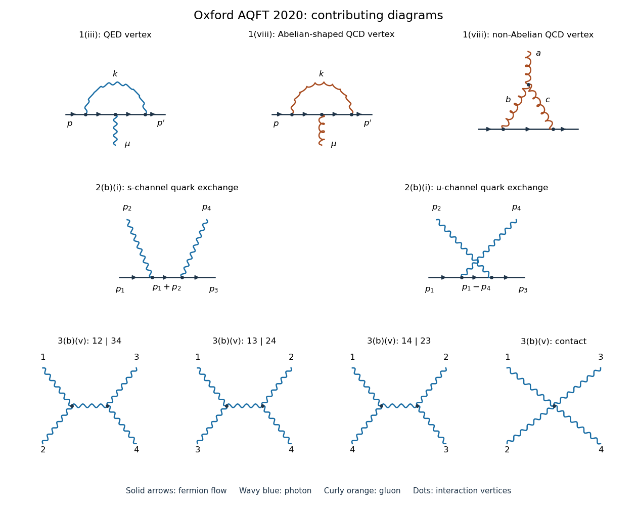
Let the bare fields obey the wave-function renormalization definitions ${\psi }_0=Z_2^{1/2}\psi$, $A_{0\mu }=Z_3^{1/2}{A}_{\mu }$, and put $m_0=Z_{m}m$. Define the vertex renormalization factor by $e_0={\mu }^{ϵ/2}e{Z}_1{Z}_2^{-1}{Z}_3^{-1/2}$. Substitution into the bare QED Lagrangian density givesEquivalently, write $Z_i=1+{\delta }_i$ and ${\delta }_m=Z_2{Z}_m-1$. The counterterm Lagrangian isFor the subsequent Feynman gauge calculation include $-(\partial \cdot A{)}^2/2$ in the gauge-fixed action. The Ward identity for QED renormalization constants implies $Z_1=Z_2$ when the regularization preserves gauge invariance; this is a consequence, rather than an extra independent definition of the renormalization constants.

The Clifford algebra of the gamma matrices gives ${\gamma }^{\nu }{\gamma }^{\mu }=2g^{\nu \mu }-{\gamma }^{\mu }{\gamma }^{\nu }$ and ${\gamma }^{\nu }{\gamma }_{\nu }=D1$. ThereforeThe contraction $g^{\nu }{}_{\nu }=D$ must be retained until the dimensional regularization calculation is complete; replacing it prematurely by four can change finite terms multiplying a ultraviolet pole.

There is one one-particle-irreducible Feynman diagram: an internal photon joins two points of the open fermion line, with the external photon attached to that line between them. It is the upper-left panel of the figure. Route internal photon four-momentum $k$ from the incoming side to the outgoing side; the adjacent internal fermion four-momenta are $p-k$ and $p^{\prime }-k$. The symmetry factor is one.

The vertex renormalization counterterm is an additional local contribution when forming the renormalized Feynman vertex. External-leg self-energy insertions belong to the complete three-point correlation function, rather than this amputated one-particle-irreducible Feynman diagram.

With $q=p^{\prime }-p$ and the routing just described, multiplication of the three QED Feynman rules for the Feynman vertices, the two Dirac propagators and the photon propagator gives $(-i{e}_D{)}^3{i}^2(-i)=-e_D^3$. Hence the unrenormalized amputated Feynman vertex through this order isFor the renormalized Feynman vertex, add $-i{e}_D{\delta }_1{\gamma }^{\mu }$ to this expression. Contributions from replacing parameters inside the one-loop term by their bare counterparts enter at higher loop order.

Keep $m>0$ and set $p=p^{\prime }=0$, which is an off shell choice. The numerator isTerms odd in $k$ integrate to zero. Lorentz covariance and dimensional regularization give, inside this integral,Applying the gamma matrices identity from part (ii) once more yieldsConsequentlyThis massive zero-momentum QED vertex integral uses an integrated tensor identity for the replacement of $N^{\mu }$, not an equality for each fixed $k$. The physical photon remains massless. The retained fermion mass supplies a scale and makes this zero-external-four-momentum calculation suitable for extracting the ultraviolet pole without a scaleless integral.

After a Wick rotation, the term in question has radial behaviorThe radial integrand is proportional to $k_E$ at the origin and to $k_E^{-3}$ at infinity. Thus it has neither an infrared divergence nor an ultraviolet divergence. In fact the area of the unit three-sphere givesThis also follows from the Feynman parameter identitywith $A=k^2+i0$, $B=k^2-m^2+i0$. Although the parameterized denominator becomes massless at $x=1$, its numerator $1-x$ cancels the apparent endpoint singularity. Since $\beta \to -2$, multiplication by $\beta$ preserves finiteness. No artificial photon mass is needed.

Only the term proportional to $\alpha$ has an ultraviolet pole. Its $k^2$ cancels the massless denominator, leaving the standard Feynman integralIn the present dimensional regularization convention, $\Gamma (ϵ/2)=2/ϵ+O(1)$ and $\alpha =1+O(ϵ)$. ThereforeThe counterterm contribution is $-i{e}_D{\delta }_1{\gamma }^{\mu }$. Cancellation of the ultraviolet pole fixeswhere the displayed expression uses the minimal subtraction scheme; a different renormalization scheme may add finite $O(e^2)$ terms. In the frequently used convention $D=4-2\epsilon$, the same result is $Z_1=1-e^2/(16{\pi }^2\epsilon )+O(e^4)$. The sign agrees with $Z_1=Z_2$ from the Ward identity for QED renormalization constants in Feynman gauge.

The proper quark-gluon vertex colour factors come from two one-particle-irreducible Feynman diagrams, shown in the upper-middle and upper-right panels. One has a virtual gluon joining the open quark line on opposite sides of the external gluon insertion. The other has two virtual gluons meeting the external gluon at a three-gluon Feynman vertex, with their other ends joined by an internal quark. A Faddeev-Popov ghost field has no direct quark coupling, so it supplies no additional one-loop Feynman vertex graph here.

Let $T^a$ be the Hermitian generators of the fundamental representation of $SU(N)$, with $\mathrm{tr}(T^a{T}^b)={\delta }^{ab}/2$, $[T^a,T^b]=i{f}^{abc}{T}^c$, ${\sum }_b{T}^b{T}^b=C_{F}1$, and $f^{abc}{f}^{dbc}=C_A{\delta }^{ad}$. Here $C_F=(N^2-1)/(2N)$ and $C_A=N$ are quadratic Casimir operators evaluated in the fundamental representation and the Adjoint representation.

For the first graph, the ordered product is ${\sum }_b{T}^b{T}^a{T}^b$. Expand the double commutator:Thus its colour factor isFor the second graph choose the orientation of the three-gluon Feynman vertex so that its group tensor is $f^{abc}$ and the ordered product along the quark line is $T^b{T}^c$. Antisymmetry removes the anticommutator part:The corresponding real group coefficient is $C_A/2=3/2$ after the conventional factor of $i$ is incorporated into the remaining Feynman rules. If the vertex is written with $i{f}^{abc}$, its raw matrix product is instead $-C_A{T}^a/2$. Reversing the ordered product reverses its sign together with the orientation-dependent three-gluon Feynman rule; these conventions describe the same scattering amplitude. External-leg corrections and local counterterms are separate from these two proper one-loop graphs.

Use the path integral with source termThe sources $\eta ,\bar{\eta }$ are Grassmann variables; all derivatives below are left functional derivatives. Because $\eta$ stands to the right of $\bar{\psi }$, differentiating with respect to it introduces a minus sign. The insertion rules are thereforeFor example ${\delta }_L(\bar{\psi }\eta )/\delta \eta =-\bar{\psi }$. The order of the odd functional derivatives matters: the rightmost derivative acts first, and the displayed product inserts ${\bar{\psi }}_{\alpha }{\psi }_{\beta }$ in that order.

Expand $\exp [-ie\int \bar{\psi }{\gamma }^{\mu }\psi A_{\mu }]$ in its power series, replace each field by its source derivative, and pull the derivatives outside the free path integral. Re-exponentiating givesThis identity concerns the unnormalized generating functional. Normalized correlation functions divide by its zero-source value so that vacuum contributions cancel.

First fix a convention that is implicit in the source. For the stated free generating functionalthe time-ordered Wick contractions are $S_F=⟨T\psi \bar{\psi }{⟩}_0=-iS$ and ${\Delta }_F=⟨TAA{⟩}_0=-i\Delta$. These follow directly by the source differentiation rules in part (i). Thus the kernels called propagators in the question are distinguished here from the contractions, which already include their factors of $i$.

At first order in the QED interaction, write $a$ for its integration point. The normalized three-point correlation function isThe zeroth-order term vanishes because the free photon one-point correlation function is zero. There are two nonzero Wick contractions of the four fields:The first term pairs the two external fermions directly and closes the two fields at the interaction into a fermion loop; its minus sign is the closed fermion loop sign. The second term joins the external fermions through the interaction, giving the connected contribution. This is also obtained by differentiating the quartic term $(i\bar{\eta }S\eta {)}^2/2$ in the free generating functional; the two choices of bilinear cancel its factor $1/2$.

Insert $S_F=-iS$ and ${\Delta }_F=-i\Delta$. Since $(-ie)(-i{)}^3=e$, the result is exactlyThe trace term is a disconnected product of a photon tadpole diagram with the free external fermion propagator; the other term is the connected three-point correlation function. In this QED calculation the disconnected term vanishes, as established next. With a convention using $S_F,{\Delta }_F$ themselves as the symbols for the propagators, the equivalent formula retains the prefactor $-ie$ and the connected-minus-trace ordering above; mixing these two conventions would give an erroneous overall phase.

The massive Dirac propagator isUse the gamma matrix trace identities $\mathrm{tr}{\gamma }^{\mu }=0$ and $\mathrm{tr}({\gamma }^{\mu }{\gamma }^{\rho })=4g^{\mu \rho }$. They giveThe integrand is odd under $k\mapsto -k$, and dimensional regularization preserves that symmetry. The same vanishing holds for $S=i{S}_F$. One must not assert that $S(0)$ itself is zero: its term proportional to $m1$ generally is nonzero and divergent, but its trace against a single gamma matrix is zero. This one-photon fermion loop is also the simplest instance of Furry's theorem.

The two tree-level Feynman diagrams are the $s$-channel and $u$-channel quark exchange graphs, drawn in the middle row of the figure. Along the directed quark line the incoming photon is absorbed before the outgoing photon is emitted in the first graph; those two insertions are reversed in the second. Their internal four-momenta are $q_s=p_1+p_2$ and $q_u=p_1-p_4$, respectively. There is no three-photon Feynman vertex in ordinary QED, and no two-photon-two-quark contact interaction in the Dirac field Lagrangian density.

Put $Q_u=2/3$, $s=q_s^2$, $u=q_u^2$, and suppress the common colour factor ${\delta }_{ji}$. Define $i\mathcal{M}$ by the product of Feynman rules. With massless external Dirac spinors the two graphs giveThe massless Dirac equation gives $/p_{1}u(p_1)=0$ and $\bar{u}(p_3)/p_3=0$. ThusBy four-momentum conservation, $p_2=p_3-q_u$, soThe two terms cancel:This is the Ward identity for the incoming photon; replacing its photon polarization vector by its four-momentum produces zero. The outgoing photon obeys the analogous identity. Each exchange graph separately fails this test, so the cancellation requires their sum. Consequently the physical scattering amplitude is invariant under ${\epsilon }^{\mu }(p_2)\mapsto {\epsilon }^{\mu }(p_2)+c{p}_2^{\mu }$.

For massless quark Compton scattering, the color average contributes one, since $(1/N_c){\sum }_{i,j}|{\delta }_{ji}{|}^2=1$. The spin average and incoming photon polarization average supply $1/(2\cdot 2)=1/4$. The Ward identities permit use of $-g_{\mu \nu }$ for each photon polarization completeness relation, and the massless fermion spin sum is ${\sum }_r{u}_r(p){\bar{u}}_r(p)=/p$.

LetReversing the gamma matrices order gives its Dirac-conjugate matrix ${\bar{A}}^{\mu \nu }$. The squared scattering amplitude isFor clarity evaluate the four traces before dividing by their denominators. The Mandelstam variables obey $s+t+u=0$, with $t=(p_1-p_3{)}^2$, $p_1\cdot p_2=s/2$, $p_1\cdot p_4=u(-1/2)$ and $p_1\cdot p_3=-t/2$. For the squared $s$-channel contribution, the gamma matrix trace identities implyHere $/q_s/p_1/q_s=2(q_s\cdot p_1)/q_s-q_s^2/p_1=s/p_2$ and $p_3\cdot p_2=-u/2$. For the squared $u$-channel contribution, $/q_u/p_1/q_u=-u/p_4$ givesOne interference trace reduces tosince $q_s\cdot q_u=(s+t+u)/2=0$. The other interference trace is its complex conjugate and also vanishes. ThereforeEquivalently $C=512{\pi }^2{\alpha }_{\mathrm{em}}^2/81$ in terms of the fine-structure constant. In the physical noncollinear region $s>0$, $u<0$, so the result is positive. The singular massless endpoint $u=0$ reflects a collinear divergence; it is not a negative squared scattering amplitude.

Goldstone's theorem states that in a relativistic quantum field theory, spontaneous breaking of an exact continuous global internal symmetry produces a massless Goldstone boson for each independent broken generator. More precisely, a conserved global current whose charge acts nontrivially on the vacuum expectation value has a massless pole in an appropriate current-field correlation function. The usual counting assumes a Lorentz invariant vacuum state and the standard locality and positivity hypotheses.

A local gauge symmetry is a gauge redundancy, so it does not by itself imply massless physical Goldstone bosons. In the Higgs mechanism, the corresponding scalar directions provide the longitudinal polarizations of massive gauge bosons.

For fundamental-doublet breaking of SU(2), assume $\lambda >0$ and $v>0$. The minima of the scalar potential satisfy ${\varphi }^{†}\varphi =v^2/2$, giving a three-sphere vacuum manifold. A chosen vacuum expectation value is ${\varphi }_0=(0,v{)}^T/\sqrt{2}$. No nonzero generator $a_a{\tau }^a$ annihilates ${\varphi }_0$: its squared norm is $v^2(a_1^2+a_2^2+a_3^2)/8$. At the group level, an $SU(2)$ matrix fixing the nonzero vector ${\varphi }_0$ must be the identity. Thus all three generators of the SU(2) gauge theory are broken in the usual perturbative Higgs mechanism description.

Make the radial and angular fields explicit:A local gauge transformation removes the three angular fields ${\pi }^a$. In unitary gauge, the Pauli matrices identity $\{{\tau }^a,{\tau }^b\}={\delta }^{ab}1/2$ givesThe mixed derivative term cancels between a term and its complex conjugate. The scalar potential becomesConsequently the complete physical Lagrangian density isReading the quadratic terms with their canonical factors $1/2$ givesAll physical scalar-vector and scalar self-interactions are displayed in the second line of $\mathcal{L}$. In particular the new cubic couplings proportional to $v$ are $h{A}^a{A}^a$ and $h^3$. Their Feynman vertices, together with the quartic ones, areThe three-vector and four-vector interactions are already contained in the non-Abelian gauge field strength term. There are no further physical fields or interactions in this specified model. Before fixing unitary gauge, the quadratic angular term is $\frac{1}{2}({\partial }_{\mu }{\pi }^a-m_A{A}_{\mu }^a{)}^2$. It exhibits three zero-curvature angular directions of the scalar potential, but also their mixing with the gauge fields. They supply the third polarization of each massive gauge boson, rather than massless physical particles.

The degrees of freedom count is $3\cdot 2+4=10$ before breaking and $3\cdot 3+1=10$ afterwards. If instead the symmetry were global, as in the decoupled $g=0$ scalar theory, the three angular fields would be physical massless Goldstone bosons. This is consistent with Goldstone's theorem. The language of a broken local symmetry refers to this gauge-fixed expansion; a gauge-dependent vacuum expectation value is not itself a gauge-invariant observable.

A gauge-invariant path integral counts all representatives of each gauge orbit. In a perturbative region with a regular gauge fixing slice, insert the Faddeev-Popov gauge-orbit identityThe Faddeev-Popov determinant is the functional Jacobian converting integration over the gauge transformation parameter into integration over the condition. The redundant gauge group volume then factors out of normalized correlation functions.

Choose $A_{\mu }^{\omega }=A_{\mu }+{\partial }_{\mu }\omega$. Its infinitesimal variation givesThere is no derivative of $A$ in this expression: only $A_{\mu }$ is varied in $A^2$. For $\lambda =0$, the determinant is field independent and can be absorbed into normalization. For $\lambda \ne 0$, it is a functional of the gauge field, so dropping it changes the path integral, even though the gauge group is Abelian. Constant residual gauge transformations are removed by boundary conditions or by dividing out their volume, as usual in perturbative gauge fixing.

An ordinary bosonic Gaussian functional integral produces an inverse determinant. An integral over independent Grassmann fields $c,\bar{c}$ instead produces a determinant, allowing a local action to represent the Faddeev-Popov determinant. With one convenient antighost sign convention,Multiplying the operator by the field-independent factor $-i$ changes only the normalization of its determinant. After integration by parts, an equivalent density isThus the Faddeev-Popov ghost fields have a massless kinetic term and a photon-ghost-antighost interaction proportional to $\lambda$. They are auxiliary anticommuting scalar fields, not physical external particles. Closed ghost loops carry the minus sign of Grassmann variables. Replacing $\bar{c}$ by $-\bar{c}$ reverses both displayed signs without changing any observable; both the kinetic and interaction conventions must be changed together.

For fixed $A$, the delta functional sets $\sigma (x)=F[A](x)$. Therefore its weighted functional integral isSince the action enters as $e^{iS}$, the gauge fixing contribution isThe Faddeev-Popov determinant does not depend on $\sigma$ and remains in the path integral. The limit $\xi \to 0$ enforces the original condition sharply; for nonzero $\xi$ this is a weighted average of the gauge slices.

Expand the gauge fixing square:The second term is a derivative cubic photon interaction; the third is a quartic photon contact interaction. Both arise from nonlinear Abelian gauge fixing, rather than an additional physical electromagnetic force.

For $\xi =1$, differentiating the quartic term with respect to four identical gauge fields gives eight copies for each pairing, henceWith the Fourier convention $A(x)=\int d^{4}p(2\pi {)}^{-4}{e}^{ipx}A(p)$ and all four-momenta incoming, the differentiated cubic term givesmatching the supplied Feynman rules. Reversing the Fourier convention reverses this cubic rule's sign; each exchange graph contains two such Feynman vertices, so its contribution is unchanged.

There are four tree-level Feynman diagrams: three photon exchange graphs with pairings $12|34$, $13|24$, $14|23$, and the four-photon contact interaction. They are drawn in the bottom row of the figure. With no external fermions or Faddeev-Popov ghost fields, an internal matter or ghost line would have to close into a loop; it cannot add a tree-level Feynman diagram here.

Use all-incoming null four-momenta $k_i$ with ${\sum }_i{k}_i=0$. Let ${\epsilon }_i$ be the external photon polarization vectors, including the complex conjugation for physical outgoing photons, and impose $k_i\cdot {\epsilon }_i=0$. For one pairing $ij|kl$, put $K=k_i+k_j=-(k_k+k_l)$. At the first cubic Feynman vertex, the terms proportional to $k_i\cdot {\epsilon }_i$ and $k_j\cdot {\epsilon }_j$ vanish, leavingAt the other end, the incoming internal four-momentum is $+K$, giving $+2\lambda ({\epsilon }_k\cdot {\epsilon }_l)K^{\sigma }$. The Feynman gauge photon propagator then givesThe last expression is evaluated at generic kinematics, with singular channel limits taken after cancellation. Summing the three pairings produces $+4i{\lambda }^{2}P$, whereThe quartic Feynman vertex contributes $i{\mathcal{M}}_{\mathrm{contact}}=-4i{\lambda }^{2}P$. ThusThis is the tree photon-scattering cancellation in a quadratic Abelian gauge: the individual gauge fixing interactions cancel in the physical scattering amplitude. The argument uses transverse external photon polarization vectors; it does not assert that an arbitrary off shell four-point correlation function vanishes. Physical light-by-light scattering first occurs through charged-particle loop Feynman diagrams.