Continuity on the compact rectangle gives finite constants and . The real mean value theorem in the second coordinate gives within the rectangle. Define the Picard iterates on the entire interval byIf the previous iterate stays in the vertical range of , then . Induction therefore makes all these iterates well defined on .
Repeated use of the Lipschitz bound gives the factorial estimateThe case is the direct integral bound; integrating the estimate for proves the next one, on either side of . The series of uniform bounds converges, so the iterates converge uniformly to a continuous function taking values within the closed vertical range. The Lipschitz estimate permits passage through the integral to give . The fundamental theorem of calculus now gives and . Thus the solution exists on the full stated interval; no extra restriction was used.
For the specified equation take , so . On ,The condition holds at , namely . The rectangle avoids , so both continuity hypotheses hold there.
Direct separation gives , hence and the initial value yields . The branch through isIt remains positive on this interval. At it reaches zero, where the differential equation is undefined, so this is its maximal real interval containing zero. The rectangle theorem supplies a sufficient interval, smaller than that actual interval.
For the particular equation, write and . Its left side is . Choose and ; these are smooth invertible coordinates in the positive quadrant, with inverse , . In them and . Subtraction of their squares leaves , so the canonical equation is . Integrating it gives .
Parameterize the data curve by , . Its coordinate values are , soDifferentiate the first identity along the curve to get . Adding gives , and then . Thus for and for . ThereforeThe coordinate rectangle gives exactly the regionIts boundary consists of up to and the ray from that point onward. It is unbounded upward. The original data curve lies inside this region. The sketch displays both characteristic boundaries and that data arc.
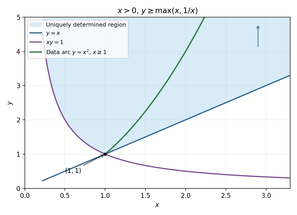
Region fixed by the partial Cauchy data and its characteristic boundaries
. Details. 
To establish the exact extent of uniqueness, outside this region either or . A smooth function supported in that unprescribed coordinate range can be added to or without changing either datum on the arc. Hence the displayed global formula is one extension, but data alone do not uniquely determine values outside the shaded region. Boundary values are fixed by continuity. The following classification criteria are pointwise and assume a nonzero principal coefficient matrix.
The principal matrix is . The equation is elliptic at a point when , equivalently the principal form has eigenvalues of the same nonzero sign and no real characteristic directions.
The equation is parabolic at a point when and at least one of is nonzero. The principal matrix then has rank one, with a repeated characteristic direction. If all three vanish, there is no second-order principal part there and the usual parabolic classification does not apply.
The equation is hyperbolic at a point when . The principal form has one positive and one negative eigenvalue and two distinct real characteristic directions. In the given equation , , , so throughout the positive quadrant, consistent with the two canonical characteristic families used above.
Under the usual existence and boundary hypotheses for the Laplace transform,The first formula requires a finite right limit and sufficient regularity for integration by parts; it is not to be applied blindly to the singular function . For that function and real , substitute :Use the second transform identity to obtain
Take the time transform of the heat equation, with differentiation and boundary limits interpreted in the standard decaying heat-solution class. The initial value is zero, so . Transforming the constant flux gives . Decay selects the decreasing solution of the transformed ordinary differential equation, givingConsequentlyThe boundary value follows by comparing with the transform of .
One can also check the decay and transform steps without relying on a merely pointwise limit under an improper integral. Using the complementary error function, the classical heat solution isDifferentiation verifies , , and for . Its integral representation gives and pointwise decay as . Thus supplies an integrable majorant, proving by dominated convergence. The same representation gives the required regularity for the transforms. This explicitly verifies that the solution selected by the decaying transformed equation lies in the intended heat-solution class.
Articles by others on the same topic
There are currently no matching articles.