Source release: Oxford examination archive, member
FOI-20210708-1 - Data/4302.pdf. The cover prints formal code 4302, paper label AC2, the title “Algebra, Analysis and Differential equations II”, and Tuesday 19 June in Trinity Term 2012.Answer availability checked on 28 October 2026: a bounded search of official Oxford sources found no advertisement of complete or selected-part solutions for this exact paper. The general advertisement of even-year solutions dating back to at least 2016 does not establish coverage of 2012.[ref]
https://www.maths.ox.ac.uk/members/students/undergraduate-courses/examinations-assessments/overview-examinations. Mathematical Institute, “Past papers and model solutions”: even-year solutions dating back to at least 2016
The minimal polynomial is the unique monic polynomial of least positive polynomial degree satisfying . Such an annihilating polynomial exists without using the Cayley-Hamilton theorem: the vector space has dimension of a vector space equal to , so are linearly dependent. Normalize a nonzero annihilating polynomial to be monic and choose one of least degree. Two distinct monic choices of that degree would have an annihilating difference of lower degree, contradicting minimality. A nonzero constant cannot annihilate because .
Choose a basis and let . The characteristic polynomial isIt is independent of the chosen basis. Indeed a change of basis replaces by a similar matrix , andby multiplicativity of the determinant. Thus this monic degree- polynomial is an invariant of the linear transformation itself.
Since is a cyclic vector and , . Finite dimension of a vector space forces a first dependence in the sequence . Let be the smallest index with in the linear span of its predecessors. Thenis linearly independent. Its linear span is invariant under : all but the last basis candidate map to the next, and the last maps to . Induction therefore puts every in . Cyclicity gives , so is a basis and .
WriteThe matrix of in this basis is the companion matrixFor , the defining relation says . Since commutes with , it also annihilates every in , hence . No nonzero polynomial of degree less than can annihilate , because that would contradict linear independence of . Thus .
Finally the characteristic polynomial of a companion matrix is , by direct determinant expansion. Explicitly, expansion along the first row of gives the recurrencestarting from . It yields . ConsequentlyThis proves that a cyclic operator has equal minimal and characteristic polynomials by the cyclic basis and a direct determinant calculation, with no appeal to the Cayley-Hamilton theorem.
For , choose the third standard basis vector . Its first three orbit vectors areThey are linearly independent: their matrix of columns has determinant . They therefore span , proving has a cyclic vector, namely .
For , write where . The binomial theorem gives for every integer . The entire orbit of any lies in , which has dimension of a vector space at most two. Therefore has no cyclic vector in the three-dimensional space. Equivalently, its minimal polynomial is , while its characteristic polynomial is .
Use the inner product convention that the first argument is linear and the second is conjugate-linear. This is the convention corresponding to the conjugated eigenvalue in part (c).
An orthonormal basis is a basis with , where is the Kronecker delta. Each vector has norm one and distinct vectors are orthogonal.
The Gram-Schmidt process starts from a basis and definesThe coefficients are in this order because the inner product is linear in its first argument. For , taking the inner product with gives . The residual cannot be zero: otherwise would belong to the linear span of , contradicting the initial basis. Normalization makes , while induction preservesThus the process produces an orthonormal basis of all of .
In an orthonormal basis, every vector has the coordinate expansion . If for all , apply it to , and take complex conjugates:ConsequentlyConversely, this formula givesLinearity in the first argument and conjugate-linearity in the second extend the equality from basis vectors to all . This proves the equivalence.
The displayed formula specifies exactly one image for each basis vector, so it defines a unique linear transformation and proves the existence and uniqueness of the adjoint on an inner product space.
Conjugate symmetry givesBy uniqueness of the adjoint operator, . Alsoso uniqueness gives . The reversal of order follows directly from moving the two factors across the inner product one at a time.
For a nonzero eigenvector of ,Therefore is real and nonnegative, and so every eigenvalue is real and nonnegative.
The preceding adjoint identities give , so this linear operator is self-adjoint. The stated finite-dimensional spectral theorem supplies an orthonormal basis with . If , thenSince ,Taking nonnegative square roots provesThe square roots of these extreme eigenvalues are the smallest and largest singular values of ; the lower bound can be zero if has a nontrivial kernel of a linear map.
An irreducible element is a nonzero nonunit such that every factorization has at least one of a unit in a ring.
A prime element is a nonzero nonunit such that implies or . Equivalently its principal ideal is a nonzero prime ideal. These are definitions in the given commutative ring; the equivalence between irreducibility and primality requires additional hypotheses on the ring.
A Euclidean domain is an integral domain with a function such that, for and nonzero , there exist with and either or . This is the Euclidean-ring convention used here.
If an ideal is zero, it is generated by zero. Otherwise choose nonzero with minimal. For any , Euclidean division gives , with . A nonzero remainder would have , contradicting the choice. Hence and . The reverse inclusion follows from , provingNow suppose is an irreducible element. Its principal ideal is proper because is not a unit. If , write by the result just proved. Then for some . Irreducibility gives either a unit, so , or a unit, so . There is no intermediate proper ideal, and therefore is a maximal ideal.
For a field , the polynomial ring is an integral domain and the polynomial division algorithm gives with or . Thus the polynomial degree is a Euclidean function, proving is a Euclidean domain.
The polynomial is irreducible over by Eisenstein's criterion with prime two: all coefficients except the leading one are divisible by two, while the constant coefficient is not divisible by four. Together with Gauss's lemma, this establishes irreducibility in . Part (b) shows that its principal ideal is a maximal ideal, soLet denote the residue class of . The polynomial division algorithm gives every residue class a representative of degree less than , so span over . If a linear combination of them vanished, its degree-less-than- representative would be a multiple of the degree- polynomial , and hence would be zero. They are therefore a basis, givingThe quadratic polynomial has no rational root, so it is irreducible over . The same maximal-ideal argument proves is a field.
These two quadratic fields are not isomorphic. In , the class of squares to . But embeds in by sending its class of to : evaluation at has kernel , by irreducibility and polynomial division. No real number squares to , so no element of does. A field isomorphism preserves one, minus one and squaring, so it cannot carry to .
The Cauchy integral formula says that if is holomorphic on the simply connected open set , and is a positively oriented simple closed curve in , then, for every in its interior,Here the contour and its enclosed region lie in ; the contour can be taken piecewise continuously differentiable. More generally, the same formula needs only holomorphic function on an open neighbourhood of that closed region. The orientation is counterclockwise, so the winding number about an interior point is one.
Write . The local maximum property gives a disk around on which , contained in the unit disk. If , then on that neighbourhood, and the identity theorem makes zero on the connected unit disk.
Otherwise multiply by the unit complex number , obtaining a holomorphic function with and nearby. Applying the Cauchy integral formula on any sufficiently small circle of radius gives the mean value propertyTake real parts. The continuous function is nonnegative on the circle and has integral zero, so it vanishes everywhere there. Since , having real part forces imaginary part zero. Thus throughout the circle. The zeros of have an accumulation point inside its domain, so the identity theorem gives constant on the entire unit disk. This proves the local maximum modulus principle directly from the Cauchy integral formula.
The closed unit disk is a compact set, and is continuous on it because is holomorphic on an open neighbourhood. The extreme value theorem therefore supplies a point where its maximum is attained. If such a point is on the boundary, the conclusion follows. If it is in the interior, part (i) makes constant on the open disk; continuity then gives the same value on the boundary. ConsequentlyThe assumption that the closed disk lies in is what makes the boundary values and the compactness argument available.
Because , the Taylor series of at zero shows thatis holomorphic throughout the unit disk. Fix . On we have , and the maximum modulus principle on the closed disk of radius gives for . For any fixed inside the unit disk we may let increase to one, obtaining . Hence the Schwarz lemma inequalities areThe derivative bound is the same estimate at , using the holomorphic extension of the quotient.
Either equality condition says that the holomorphic function from part (i) has modulus one at an interior point: at zero in the derivative case, or at the given nonzero point in the other case. Since everywhere, the maximum modulus principle makes a constant with . ThereforeThese maps are rotations of the unit disk and do achieve both equalities, so this also identifies all equality cases of the Schwarz lemma.
The Laurent theorem states that a holomorphic function on the annulus has a unique Laurent seriesThe integration circle is counterclockwise. The series converges absolutely at every point of the annulus and uniformly on every compact subannulus. The coefficient integrals are independent of the choice of by the Cauchy integral theorem applied between two such circles. These statements include or when the indicated annulus has those endpoints.
An isolated singularity at means that some radius has holomorphic on the punctured disk , while is not initially defined as a holomorphic function at . The adjective isolated refers to the absence of other singularities in this punctured neighbourhood; it permits a removable singularity.
The point is a removable singularity if assigning a value to makes holomorphic on a full neighbourhood of . Equivalently, its Laurent series has no nonzero coefficients of negative powers. The assigned value is its constant coefficient, or equivalently the finite limit .
A pole of order meansEquivalently, the Laurent series has a finite nonzero principal part, with lowest power exactly . Thus extends holomorphically with nonzero value at ; using a smaller positive power would not remove the singularity.
An essential singularity is an isolated singularity that is neither a removable singularity nor a pole. In its Laurent series, infinitely many coefficients of negative powers are nonzero. The alternatives follow because no negative terms give a removable singularity, while finitely many with a lowest nonzero power give a pole.
Inside the unit circle, use the geometric series for :Outside the unit circle, expand in powers of instead:The different Laurent series reflect different annuli separated by the pole at one. Both follow from absolutely convergent geometric series in their stated regions.
Take the Laurent series of on . For every integer , its coefficient of satisfies, on a circle of radius ,The coefficient is independent of . Letting therefore gives for every . The Laurent series is a power series with no negative powers and supplies a holomorphic extension at zero. Thus zero is a removable singularity. This is the Riemann removable singularity theorem, with boundedness used to eliminate the entire principal part.
Suppose, towards a contradiction, that for some the punctured-disk image misses the open disk of radius about . Thenis holomorphic and bounded by on . Part (i) extends it to a holomorphic function on the full disk. If , then extends holomorphically at zero, making zero a removable singularity.
If , the function is not identically zero, since it is nonzero on the punctured disk. The Taylor series and identity theorem give a finite zero order , so with holomorphic and . Hencehas a pole of order . Both alternatives contradict an essential singularity. ConsequentlyThis is the Casorati-Weierstrass theorem: every complex value can be approximated arbitrarily closely in every punctured neighbourhood of an essential singularity.
The tangent half-angle substitution maps to , withBecause , both and are positive. ThusEvaluating the improper integral givesAlthough the change of variable has an infinite endpoint, the original integrand is continuous on the closed interval, and the transformed integrand decays as , so the limiting substitution is justified.
Use the branch of the complex logarithm with , so the branch cut is the positive real axis, and take on the same slit plane. Apply the residue theorem toon a positively oriented keyhole contour with inner radius and outer radius . The upper bank travels from to , the large circle counterclockwise, the lower bank from to , and the small circle clockwise. One may first keep the banks at small nonzero angles and then take their limits.
On the upper bank, and is positive. On the lower bank, the corresponding limits are and . Reversing the lower-bank orientation therefore makes the sum of the bank integrals tend toBoth are absolutely convergent: near zero compare with , and near infinity with . On the large circle, , so its contribution is . On the small circle it is . Both tend to zero.
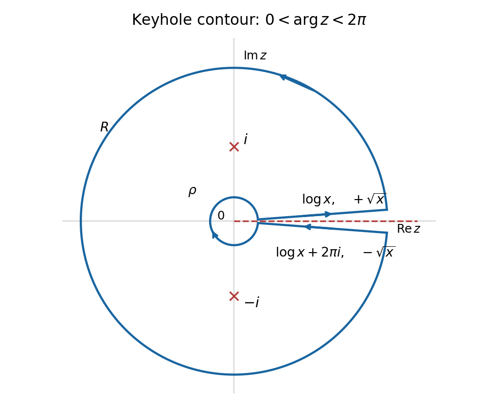

The two simple poles are and . On the chosen branch their arguments are and , respectively. Consequently their residues areFor example, the first follows from , and the derivative of the denominator factor . The second uses , rather than the value from the principal square-root branch. Adding and applying the residue theorem yieldsAs is real, taking real parts givesThe imaginary part also gives , an independent consistency check on the orientation and branch factors.
A critical point of a dynamical system or equilibrium is a point with , so the constant function is a solution. Put , . For a continuously differentiable vector field, its linearization iswith remainder in the original nonlinear system. For distinct eigenvalues, is diagonalizable over , and the linear solutions are combinations of , where are corresponding eigenvectors. Real parts determine growth or decay; nonzero imaginary parts give rotation. For hyperbolic equilibria, meaning no eigenvalue has zero real part, the Hartman-Grobman theorem transfers the local stability and qualitative orbit pattern to the nonlinear system. A purely imaginary pair is not hyperbolic: it determines a linear centre, while higher-order terms decide whether the nonlinear system actually has a centre.
A stable node hasBoth exponential modes decay as , so the equilibrium is asymptotically stable. Generic linear orbits approach tangent to the eigenvector for the less negative eigenvalue; the eigenvector directions themselves are invariant straight lines. There is no rotation because both eigenvalues are real.
An unstable node hasBoth linear modes grow forward in time. Nearby nonconstant orbits move away from the equilibrium, and approach it under reversed time; their local directions come from the two real eigenvectors.
A saddle equilibrium hasThe negative eigenvalue gives a stable manifold direction and the positive eigenvalue an unstable manifold direction. Perturbations along the latter grow, so the equilibrium is unstable even though there are special trajectories approaching it.
A centre equilibrium of the linearized real planar system hasAfter a real invertible linear change of coordinates, the system is a constant angular rotation. Its nonzero orbits are ellipses of period , so it is stable but not asymptotically stable. This is a classification of the linearization: a centre in the linearization need not be a nonlinear centre. In particular, imaginary eigenvalues alone do not prove a nonlinear centre equilibrium, which requires a punctured neighbourhood filled with periodic orbits. Part (c) illustrates exactly this limitation.
A stable spiral has the complex conjugate eigenvaluesIn suitable real coordinates the radius decays like while the angle changes at rate . The orbit therefore spirals towards the equilibrium, which is asymptotically stable. This is also called a stable focus.
An unstable spiral hasRotation is accompanied by exponentially increasing radius in suitable real coordinates. Thus nearby nonconstant orbits spiral away, and the equilibrium is unstable. This is also called an unstable focus.
The first component of the vector field vanishes only when or . The second vanishes only when or . Intersecting these alternatives gives exactly five equilibria. Their Jacobian matrix isAt ,The real parts are negative and the imaginary parts are nonzero, so is a stable spiral.
At ,so is a saddle equilibrium. All five equilibria are hyperbolic, so these linear classifications determine their nonlinear local stability as well.
The Bendixson-Dulac theorem states that if is a continuously differentiable planar vector field on a simply connected open region , and a continuously differentiable Dulac function makeshave one weak sign throughout , without vanishing identically on any nonempty open subset, then there is no nonconstant periodic orbit contained in . To see why, a hypothetical simple periodic orbit bounds a region in . The divergence theorem gives the integral of this expression as the outward flux of across the orbit. The flux is zero because the vector field is tangent to its orbit, whereas the one-sign area integral is nonzero, a contradiction. The usual stricter version assumes a strictly positive or strictly negative expression everywhere.
For the printed polynomial system, the origin is an equilibrium andThus its linearization is a centre equilibrium. For the full system take . The divergence isOn the open disk this is nonpositive, and is negative wherever . Its zero set inside the disk is a line, so it cannot vanish on any open subset. The Bendixson-Dulac theorem therefore provesThis also exposes a terminology problem in the source: a nonlinear centre equilibrium has surrounding closed orbits, so the printed claim of a centre cannot hold in that sense. The imaginary eigenvalues establish only a centre of the linearized system. In fact the full equilibrium is an asymptotically stable weak focus, as the following direct check shows.
A quartic Lyapunov correction for a weak focus makes the nonlinear damping visible. Put and consider the Lyapunov functionIt is positive definite sufficiently close to zero. Differentiating along the polynomial vector field givesFor clarity, the quartic terms come from in the derivative of , and from applying to the quartic correction. Their sum is ; all other terms have degree at least six. Therefore in a sufficiently small punctured neighbourhood, proving asymptotic stability by Second Lyapunov theorem. Finallyso nonconstant nearby orbits turn clockwise as they converge. The equilibrium is a weak focus despite the centre in its linearization. This interpretation resolves both the local dynamics and the absence of closed orbits without changing the printed coefficients.
For the linear differential operator , the characteristic equation is , with roots . Take the fundamental system of solutionsThe Wronskian is never zero, so variation of parameters is valid on the whole interval. Write a particular solution as , and impose the auxiliary condition . Substitution then gives . These two equations giveChoosing both integrals to start at zero makes the resulting particular solution and its first derivative vanish there:A general solution is . The boundary condition at zero sets . The condition at givesbecause and . Combining the two integrals yields the Green's function representationIndeed, for the kernel is , since ; for it is .
For fixed interior , the Green's function vanishes at both endpoints, is continuous at , solves the homogeneous equation away from , and satisfiesThis derivative jump is the normalization required by the leading coefficient one in . Finally, a homogeneous solution satisfying the first boundary condition is , and the second boundary condition at forces . Thus the boundary value problem has exactly one solution for every continuous forcing, justifying the unique inverse represented by this kernel.
For this forcing the integral in part (a) simplifies toConsequently the unique boundary value problem solution isIt vanishes at zero and at . To check the differential equation directly, set . Then . For , one has , as required.
The same variation of parameters construction works on . All solutions satisfying the boundary condition at zero have the formAt , the homogeneous term vanishes for every ; it can no longer be chosen to correct the final boundary value. Since , that boundary value is zero exactly whenThis condition is necessary by the displayed general solution, and sufficient by the same formula. When it holds, the full answer isFor complex-valued forcing, allow instead. The freedom is addition of the nonzero homogeneous Dirichlet solution . At this endpoint separation, the homogeneous boundary problem has a nonzero solution. The resulting Fredholm solvability condition restricts the forcing to the compatible functions described above. In the language of the Fredholm alternative, the condition is orthogonality to the adjoint null solution of with zero endpoint values.
For a quasilinear partial differential equation, the characteristic equations for a quasilinear equation are the ordinary differential equationsA solution surface is locally a differentiable graph whose tangent plane contains the vector at every point. Its normal is , so the tangency condition is precisely . Thus every characteristic lying on that graph follows the vector field without leaving the graph.
Parameterize the given initial curve by . For each , solve the characteristic equations for a quasilinear equation with initial value at . The resulting map sweeps out a candidate solution surface. If the coefficients and initial data are continuously differentiable, the Picard-Lindelöf theorem supplies this local family. To make it a graph we also need the projection to be locally invertible. At its Jacobian determinant isThe Noncharacteristic Cauchy data condition is . The inverse function theorem then gives and , and hence . Its derivatives obey the PDE by the chain rule. The same characteristic initial-value uniqueness gives local uniqueness of this solution wherever the projection remains invertible and the relevant characteristic meets the prescribed data.
The characteristic equations for a quasilinear equation here areSuccessive integration gives the general characteristicwhere are integration constants. Equivalently and are constant along each curve: differentiating them with respect to gives zero. Three constants occur because shifting the origin of the parameter describes the same geometric curve again; there are two independent curve invariants.
Use to label the initial half-line, with at . In the general characteristic from part (i), this sets , , . The parametric solution surface is thereforeAt this recovers exactly the given data. Moreover , so the surface follows the required characteristic vector field. The branch defining a classical graph through the data is determined below by restricting to the side of the projection fold containing .
For fixed , eliminate to obtain the projected parabolaAlong that curve,Equality occurs at , where the point is . Also there, so the tangent line has the same slope as the line and passes through a point of that line. Thus every projected characteristic is tangent to that line, with no crossing of it. Because , the attained tangency points form only the half-line , .
Differentiating the projected parameterization givesIt vanishes exactly when . The image is the tangency half-line from part (iii), , , . This is a fold caustic: the parameterized surface itself remains regular, but its projection ceases to be locally invertible, so it cannot there be expressed as a differentiable single-valued graph over the plane.
Put . The identity gives , and hence . On the initial half-line and the prescribed value is , which selects the positive sign. The branch containing the data has , soFor , its derivatives are . Substitution checks the partial differential equation:On the data , the value is one. The other algebraic branch gives there and does not meet these data. The positive-branch formula defines a solution on the larger half-plane , but the part uniquely fixed by the prescribed half-line also requires a nonnegative characteristic footpoint , as part (vi) explains.
Articles were limited to the first 100 out of 539 total.
Articles by others on the same topic
There are currently no matching articles.