Source: Mathematics release, supplied bundle
Part A 2007 11-1.pdf, pages 125–131. The seven-page paper is dated 23 June 2009 and serves Mathematics and Mathematics & Statistics Part A. Full source statements are retained in the private editable transcription.Bounded exact-paper checks found no matching advertisement of worked answers. Every printed task and surrounding unnumbered request is covered, with explicit qualifications for the two source formula conventions noted below.
If , then has nonzero kernel of a linear map. A nonzero vector in that kernel of a linear map satisfies , proving that is an eigenvalue. Extend to a basis. Its first column is , so the matrix has block formHere represents the induced operator on .
If the algebraic multiplicity is , repeat this argument in that quotient: its characteristic polynomial still has with multiplicity . Induction and lifting a quotient basis gives a basis whose first columns have the prescribed upper-triangular form. With the span of those vectors, the full matrix isThus is invariant and is contained in . Conversely, if , project to . The induced map is invertible, so its th power cannot kill a nonzero class. Hence . Consequently ; this proves simultaneously that it is a subspace and -invariant. It also proves on this space, without using Cayley-Hamilton theorem in advance.
To prove independence of the different spaces, take a relation with . Fix and apply . It kills all terms except . On , each factor is invertible: its inverse is a finite geometric series in the nilpotent . Hence implies . The sum is direct, and its dimension is , soFinally kills each summand, hence every vector. This proves without circularly assuming the theorem during the decomposition.
The orthogonal complement is . Put , so . Orthonormality gives , and therefore . Also for every , so . Every is thus a sum from and , and their intersection is zero, since a vector orthogonal to itself has squared norm zero. This proves . The decomposition is unique, so its two projection maps depend only on , not on the chosen orthonormal basis.
Finite dimensionality of cannot simply be dropped. Take the real Hilbert space and , the finitely supported sequences. This is an infinite-dimensional proper subspace. A vector orthogonal to every coordinate unit vector is zero, so . Yet, for example, belongs to . Hence . The failure occurs even though itself is complete; the proper dense subspace is not closed.
For any , the decomposition is orthogonal. The Pythagorean identity givesEquality is attained at . Thus , and the minimizer in is uniquely .
The assumption means . For every unit vector , orthogonality and Cauchy–Schwarz give . Equality is attained atEquality in the real Cauchy–Schwarz inequality requires to be a scalar multiple of , and attaining the positive supremum fixes its sign; the unit norm fixes its magnitude. This proves uniqueness.
Use ordinary matrix addition and multiplication on . Sums and products of polynomials in remain such polynomials, and they commute because powers of the same matrix commute. The identity is . Evaluation is a surjective unital algebra homomorphism over . It is unique among maps fixing the scalar matrices and sending to .
The scalar condition is needed for the word “unique”: as an unrestricted ring-homomorphism assertion over an arbitrary field, prescribing only the image of does not suffice. For example, over with a real scalar matrix , conjugating every coefficient gives another unital ring homomorphism with the same image of . The intended polynomial-evaluation map is the -algebra map just defined.
The kernel of a ring homomorphism is an ideal of the principal ideal domain . It is nonzero because finitely many powers of must become linearly dependent in the finite-dimensional matrix space. Its unique monic generator is precisely the minimal polynomial : division by shows that a polynomial killing has zero remainder, by minimality. Hence and .
If , Bézout's identity gives ; evaluation gives . Conversely an inverse in has form , so , which forces . Thus invertibility in this ring is exactly coprimality with the minimal polynomial.
The displayed matrix is block diagonal with a block and a block having characteristic polynomial . The latter block is not scalar, so its minimal polynomial has degree two and is exactly that polynomial. Taking the least common multiple of the block minimal polynomials gives over .
Ideals of correspond to ideals of containing , namely the principal ideals generated by the monic divisors of . Every one of the three distinct linear factors may be included or omitted, soThis includes both the zero ideal and the whole ring. Equivalently the Chinese remainder theorem identifies this ring with .
Reduce the matrix modulo two. It is , so but . Thus the minimal polynomial is . Its monic divisors are , giving exactly in the quotient.
This ring has the four elements . Coprimality with is equivalent to the representing polynomial taking value one at . Thus precisely and are units: . Indeed , whereas .
Laurent's theorem states that a holomorphic function on has a unique expansion , converging absolutely there and uniformly on compact subannuli, withHere has a simple zero at zero and no other zero in . Hence has only a simple pole there, giving the stated series with no powers below . Multiplying by and comparing the constant, linear and quadratic coefficients yields
Use the coefficient integrals on the two circles. The annular region between them contains exactly the simple poles , and the residue of at each is . Apply the residue theorem to between the circles:For lower indices, set because the inner Laurent series has no such terms; the same contour argument then still applies. Since is odd, its even-index coefficients vanish. A complete explicit list for the requested range isThe subtraction accounts for the two poles crossed; using the inner coefficients unchanged outside their annulus would miss precisely these terms.
For , integrate over the upper semicircle of radius . The arc tends to zero, since there and the denominator is of order . The sole pole is , of residue , so the real part gives . The integrand defining is even in , and by the arctangent integral. Hence
For use with a small clockwise semicircular indentation above zero. Its residue at zero is one, so the small arc tends to . The pole has residue , and the large arc again vanishes. ThusThe imaginary part is the ordinary convergent integral : its apparent singularity at zero is removable, with limit , and its tails are absolutely integrable. Therefore for . Oddness in and the value zero at give
Differentiation is valid at every real , including zero. Indeed the mean value theorem bounds the absolute difference quotient of with respect to by , an integrable majorant independent of . Dominated convergence therefore gives . In particular both one-sided derivatives at zero equal .
The complex fundamental theorem of calculus says that for a holomorphic antiderivative and a piecewise path from to , one has . The integral is therefore zero on a closed path; the antiderivative need only be defined on a neighborhood of that path, rather than on all its interior.
The assumptions make holomorphic near . Differentiate:Integrate this derivative around the closed path to obtain
For a positively oriented simple closed piecewise smooth curve, a point inside it and a function holomorphic on a neighborhood of the curve and its interior, Cauchy's differentiated integral formula isThe printed denominator uses while the derivative and factorial use . The standard formula requires these indices to agree; the intended exponent in this display is . The private transcription preserves the mismatch exactly.
For the following task, write near zero with . Thus extends holomorphically at zero, and is holomorphic inside the specified contour because has no other zeros there. Now . Apply the correctly indexed formula with derivative order to getPositive winding one supplies the orientation and multiplicity used in this expression.
Choose a small positively oriented circle in within the convergence disk of the inverse series. Cauchy's coefficient formula givesLet . The biholomorphism property makes it a simple positively oriented closed curve about zero. Under , and , soThe last equality is (a). Apply (b), givingThis is the local Lagrange inversion theorem; the simple zero ensures that the expression being differentiated has a removable singularity and a nonzero value at zero.
Continuity on the compact rectangle gives finite constants and . The real mean value theorem in the second coordinate gives within the rectangle. Define the Picard iterates on the entire interval byIf the previous iterate stays in the vertical range of , then . Induction therefore makes all these iterates well defined on .
Repeated use of the Lipschitz bound gives the factorial estimateThe case is the direct integral bound; integrating the estimate for proves the next one, on either side of . The series of uniform bounds converges, so the iterates converge uniformly to a continuous function taking values within the closed vertical range. The Lipschitz estimate permits passage through the integral to give . The fundamental theorem of calculus now gives and . Thus the solution exists on the full stated interval; no extra restriction was used.
For the specified equation take , so . On ,The condition holds at , namely . The rectangle avoids , so both continuity hypotheses hold there.
Direct separation gives , hence and the initial value yields . The branch through isIt remains positive on this interval. At it reaches zero, where the differential equation is undefined, so this is its maximal real interval containing zero. The rectangle theorem supplies a sufficient interval, smaller than that actual interval.
For the particular equation, write and . Its left side is . Choose and ; these are smooth invertible coordinates in the positive quadrant, with inverse , . In them and . Subtraction of their squares leaves , so the canonical equation is . Integrating it gives .
Parameterize the data curve by , . Its coordinate values are , soDifferentiate the first identity along the curve to get . Adding gives , and then . Thus for and for . ThereforeThe coordinate rectangle gives exactly the regionIts boundary consists of up to and the ray from that point onward. It is unbounded upward. The original data curve lies inside this region. The sketch displays both characteristic boundaries and that data arc.
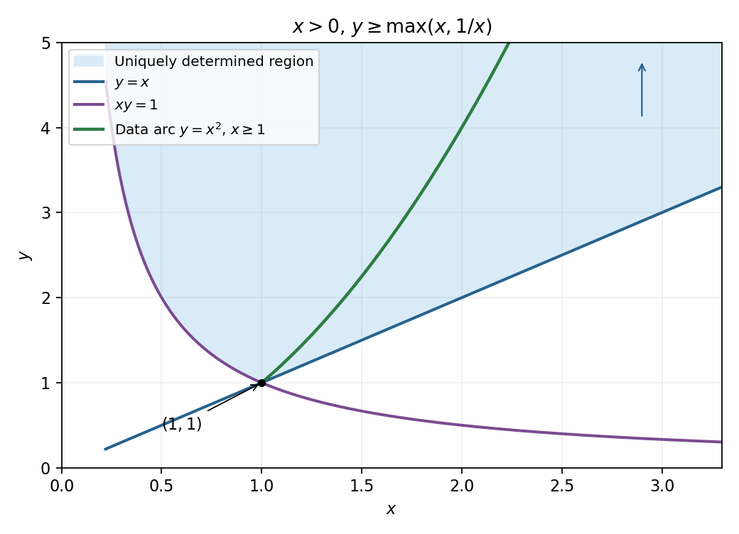
Region fixed by the partial Cauchy data and its characteristic boundaries
. Details. 
To establish the exact extent of uniqueness, outside this region either or . A smooth function supported in that unprescribed coordinate range can be added to or without changing either datum on the arc. Hence the displayed global formula is one extension, but data alone do not uniquely determine values outside the shaded region. Boundary values are fixed by continuity. The following classification criteria are pointwise and assume a nonzero principal coefficient matrix.
The principal matrix is . The equation is elliptic at a point when , equivalently the principal form has eigenvalues of the same nonzero sign and no real characteristic directions.
The equation is parabolic at a point when and at least one of is nonzero. The principal matrix then has rank one, with a repeated characteristic direction. If all three vanish, there is no second-order principal part there and the usual parabolic classification does not apply.
The equation is hyperbolic at a point when . The principal form has one positive and one negative eigenvalue and two distinct real characteristic directions. In the given equation , , , so throughout the positive quadrant, consistent with the two canonical characteristic families used above.
Under the usual existence and boundary hypotheses for the Laplace transform,The first formula requires a finite right limit and sufficient regularity for integration by parts; it is not to be applied blindly to the singular function . For that function and real , substitute :Use the second transform identity to obtain
Take the time transform of the heat equation, with differentiation and boundary limits interpreted in the standard decaying heat-solution class. The initial value is zero, so . Transforming the constant flux gives . Decay selects the decreasing solution of the transformed ordinary differential equation, givingConsequentlyThe boundary value follows by comparing with the transform of .
One can also check the decay and transform steps without relying on a merely pointwise limit under an improper integral. Using the complementary error function, the classical heat solution isDifferentiation verifies , , and for . Its integral representation gives and pointwise decay as . Thus supplies an integrable majorant, proving by dominated convergence. The same representation gives the required regularity for the transforms. This explicitly verifies that the solution selected by the decaying transformed equation lies in the intended heat-solution class.
Articles by others on the same topic
There are currently no matching articles.