Past exam of the differential equations 2 course of the University of Oxford / 2015 / 1

On an interval with $x>0$, use the power-law ansatz $y=x^r$. Substitution gives $r(r-1)+2r+1=r^2+r+1=0$, whose roots are $r=-1/2\pm i\sqrt{3}/2$. Taking real and imaginary parts of $x^r$ givesThese two real solutions are linearly independent: their Wronskian is $(\sqrt{3}/2)x^{-2}\ne 0$. They therefore span the solution space of the second-order linear ordinary differential equation on that interval.

For $x<0$, replace $x^{-1/2}$ by $|x{|}^{-1/2}$ and $\log x$ by $\log |x|$, with independent real constants on the negative interval. This follows equally by the change of variable $t=\log |x|$, which turns the Cauchy-Euler equation into $d^{2}y/d{t}^2+dy/dt+y=0$. The coefficient of $y^{\prime \prime }$ vanishes at zero, so the general formula is stated separately on either side. Every nonzero mode has an unbounded oscillatory envelope as $x\to 0$; a continuous extension through zero requires the solution to vanish identically on both sides.

Use the usual inner product $⟨u,v⟩={\int }_0^1\overline{u}vdx$. Moving four derivatives by integration by parts leaves $L^{\ast }=D^4+1$ and gives the fourth-order boundary identityThus the differential expression is formally self-adjoint. If both functions satisfy the clamped boundary conditions, every displayed endpoint product vanishes, proving symmetry on the specified domain.

To check full self-adjointness, also identify the adjoint domain. Allow $v$ to run through the clamped domain. At either endpoint, $v^{\prime \prime }$ and $v^{\prime \prime \prime }$ can be chosen independently, for instance using a polynomial near that endpoint multiplied by a smooth cutoff function. The remaining boundary form is $[\overline{u}{v}^{\prime \prime \prime }-\overline{u^{\prime }}{v}^{\prime \prime }{]}_0^1$. It vanishes for every such $v$ precisely when $u=u^{\prime }=0$ at both endpoints. These are exactly the original boundary conditions. On the regular finite interval, the adjoint domain consequently equals $\{u\in H^4(0,1):u(0)=u^{\prime }(0)=u(1)=u^{\prime }(1)=0\}$, rather than a larger domain. Here $H^4$ is the Sobolev space of functions whose weak derivatives through order four are square-integrable.

The operator together with these boundary conditions is fully self-adjoint. As a further consistency check, integration by parts gives $⟨y,Ly⟩={\int }_0^1(|y^{\prime \prime }{|}^2+|y{|}^2)dx>0$ for every nonzero admissible $y$. The reusable calculation is the Lagrange identity for a fourth-order differential operator.

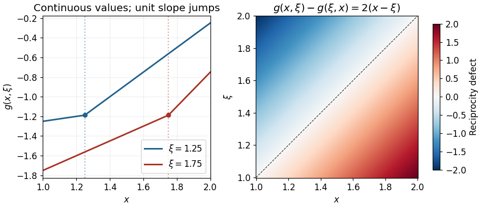
Start with a fundamental solution of the second derivative operator:Here $H$ is the Heaviside step function and the last equality holds in the sense of distributions. The factor $x-\xi$ removes a jump in the function itself, while its first derivative has a unit jump. Adding any homogeneous solution preserves the Dirac delta source.

Choose $y_1(x)=x-2$ and $y_2(x)=x-3$. They are independent homogeneous solutions, with $B_1{y}_1=0$, $B_2{y}_2=0$, $B_1{y}_2=-1$, and $B_2{y}_1=1$. Since $1<\xi <2$, the fundamental solution has $B_1\tilde{g}=1$ and $B_2\tilde{g}=2-\xi$. Imposing the two boundary conditions on the proposed combination therefore gives $-A_2+1=0$ and $A_1+2-\xi =0$. ConsequentlyEquivalently,At $x=\xi$ both expressions equal ${\xi }^2-3\xi +1$ and the right slope minus the left slope is $\xi -(\xi -1)=1$. At the endpoints, $g(1,\xi )=-\xi$ and $g_x(2,\xi )=\xi$, while $g_x(1,\xi )=\xi -1$ and $g(2,\xi )=1-\xi$. These explicitly verify both coupled boundary conditions. The homogeneous equation has only affine solutions; its two boundary conditions give $2a+b=3a+b=0$, hence $a=b=0$, proving uniqueness of the Green function.

The reciprocity defect is $g(x,\xi )-g(\xi ,x)=2(x-\xi )$. It records how the coupled boundary conditions affect self-adjointness, even though the differential expression $D^2$ is formally self-adjoint. The construction is an instance of the boundary-matrix construction of an ordinary differential Green function.