Past exam of the differential equations 2 course of the University of Oxford / 2021 / 3 / c

Setting $ϵ=0$ gives the reduced first-order linear differential equation $y^{\prime }=y$. Its nonzero solutions cannot satisfy the zero value at $x=2$, so one endpoint needs a boundary layer. To determine which endpoint, freeze the coefficient at $x=x_b>0$ in the rapidly varying part: $ϵy^{\prime \prime }-x_b{y}^{\prime }=0$ has fast mode $e^{x_b(x-x_b)/ϵ}$. It decays into the interval from the right endpoint but grows into the interval from the left endpoint. HenceThe dominant balance $ϵ/{\delta }^2\sim x_b/\delta$ gives $\delta \sim ϵ/x_b$, so a convenient local thickness is $ϵ/2$. The left boundary condition must select the outer solution. Equivalently, a putative left inner variable $X=(x-1)/ϵ$ would give $Y_{XX}-Y_X=0$, whose nonconstant solution grows like $e^X$ and cannot satisfy the asymptotic matching condition as $X\to \infty$.

The reduced equation and the left boundary condition give the leading outer solutionIntroduce the right inner variable $X=(2-x)/ϵ\ge 0$ and write $Y(X)=y(2-ϵX)$. The chain rule gives $y^{\prime }=-Y_X/ϵ$ and $y^{\prime \prime }=Y_{XX}/{ϵ}^2$. Multiplying the rescaled differential equation by $ϵ$ gives the exact equationAt leading order, $Y_{0,XX}+2Y_{0,X}=0$, with general solution $Y_0=A+B{e}^{-2X}$. The right boundary condition gives $Y_0(0)=0$. The asymptotic matching condition in the overlap region $ϵ\ll 2-x\ll 1$ givesThus $A=e$ and $B=-e$, yielding the leading inner expansionEquivalently, the inner variable $\xi =2(2-x)/ϵ$ gives $Y_0=e(1-e^{-\xi })$. Both normalizations describe the same boundary layer.

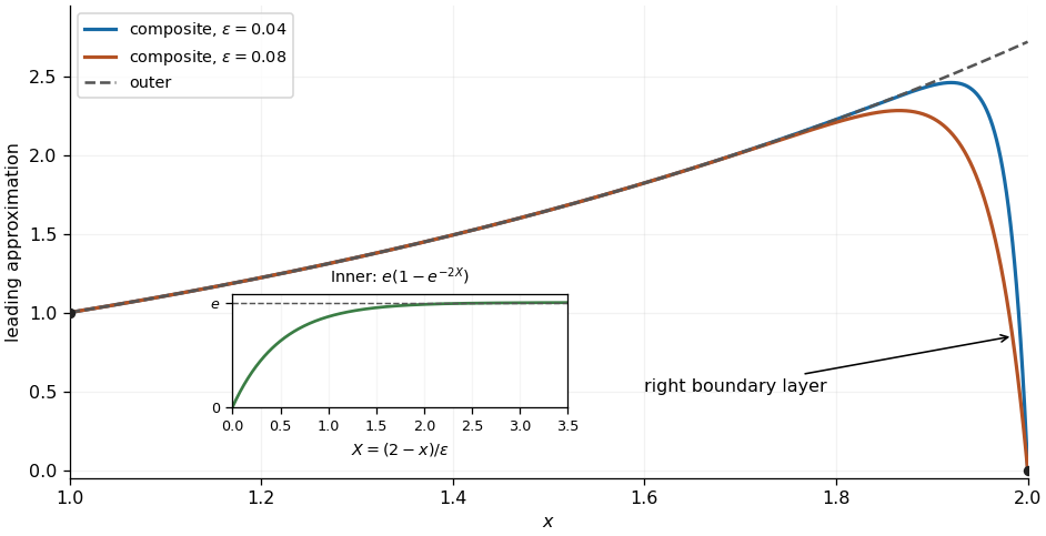
The common value in the overlap region is $e$. The additive composite expansion therefore givesThis leading approximation has $y_{\mathrm{comp},0}(2)=0$ and $y_{\mathrm{comp},0}(1)=1-e^{1-2/ϵ}$; the left endpoint error is exponentially small. It rises from near one following the outer solution $e^{x-1}$, approaches a value close to $e$, then drops rapidly to zero in the right boundary layer. Its first derivative isFor small $ϵ$ the largest value lies slightly inside the interval. For this additive composite expansion, the first derivative vanishes atThis locates the rounded top of the sketch; the rapid final drop has the $O(ϵ)$ scale found above. The additive composite expansion is a leading approximation, so its exponentially small endpoint error does not imply an exponentially small error throughout the interval: neglected algebraic corrections to the outer expansion and inner expansion remain.