The function is an odd function, passes through , and has the horizontal asymptote at both infinities. Its derivative isIt decreases for and increases for , with its lowest value and highest value . These features determine the graph of a function shown below.
For , the equation is the quadratic equation . The quadratic formula gives exactly two real equation roots:The binomial series gives , hence the two requested asymptotic expansions areTheir product is exactly one. Both are positive, with ; there are no negative equation roots because for . At the two real equation roots coincide at one, and for there are none. In the stated limit , these two branches are therefore exhaustive.
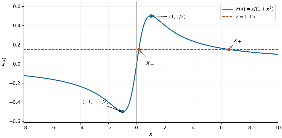
Two positive intersections of the rational function with a small positive level
. Original sketch of with the two real equation roots marked for . The curve also shows its negative lowest point and positive highest point. Details.
The power-law ansatz givesSince , the equation roots and are distinct. The Cauchy-Euler equation therefore has general solutionFor , the first derivative and second derivative areThe strictly convex function diverges to as , passes through , and has a unique lowest point atAs , , so the line is an asymptote. When , the lowest point is to the right of one; at it is at one, and for it is to the left of one.
The ratio of the two terms isThus is larger for , the terms are equal at , and is larger for . In the stronger asymptotic sense as , dominates at each fixed , and dominates at each fixed . Their crossover has , equivalently , as described by the power-law crossover in a singular perturbation. In that region with bounded gives .
Substitute the proposed regular perturbation into the differential equation. The leading and subsequent equations areConsequently , and in fact each successive coefficient has the form , because the preceding second derivative is zero. The leading approximation is thereforeIt has only one adjustable constant and generally cannot impose two independent boundary conditions. Those assumed in the question require a nonzero coefficient, which a power series in cannot recover: at fixed it is exponentially small, and at fixed it grows without bound as . Thus the regular perturbation describes the specified solution only in the region to the right of the crossover, away from ; it is not a uniform approximation on .
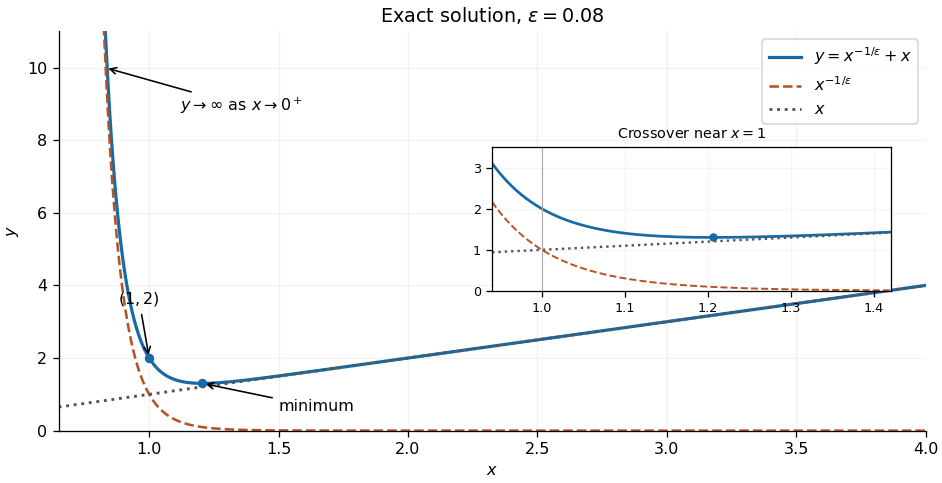
The exact solution and its two power-law contributions
. Original sketch for , showing the decreasing contribution, the increasing contribution, their sum, and its lowest point. The inset resolves the region where both terms contribute. Details.
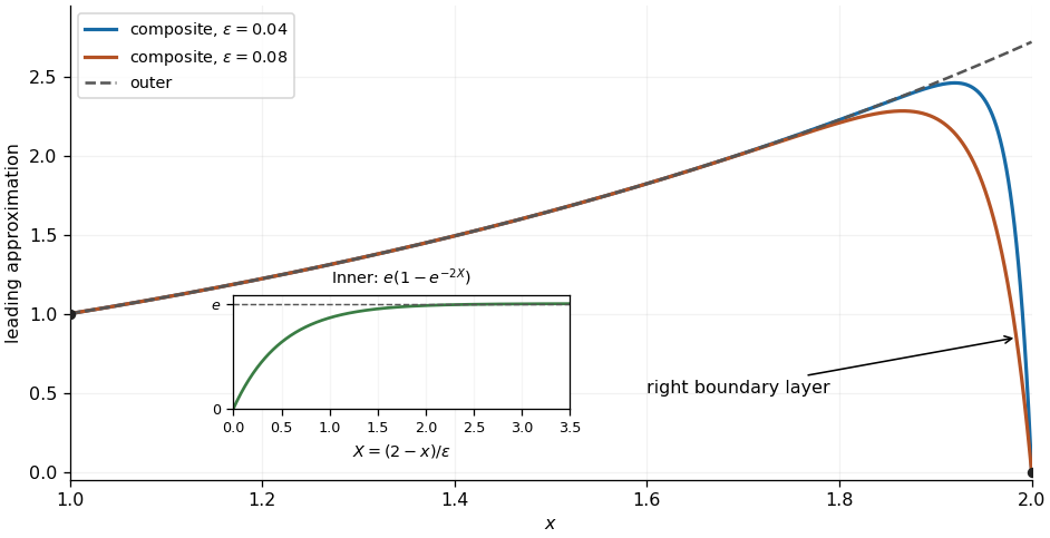
Setting gives the reduced first-order linear differential equation . Its nonzero solutions cannot satisfy the zero value at , so one endpoint needs a boundary layer. To determine which endpoint, freeze the coefficient at in the rapidly varying part: has fast mode . It decays into the interval from the right endpoint but grows into the interval from the left endpoint. HenceThe dominant balance gives , so a convenient local thickness is . The left boundary condition must select the outer solution. Equivalently, a putative left inner variable would give , whose nonconstant solution grows like and cannot satisfy the asymptotic matching condition as .
The reduced equation and the left boundary condition give the leading outer solutionIntroduce the right inner variable and write . The chain rule gives and . Multiplying the rescaled differential equation by gives the exact equationAt leading order, , with general solution . The right boundary condition gives . The asymptotic matching condition in the overlap region givesThus and , yielding the leading inner expansionEquivalently, the inner variable gives . Both normalizations describe the same boundary layer.
The common value in the overlap region is . The additive composite expansion therefore givesThis leading approximation has and ; the left endpoint error is exponentially small. It rises from near one following the outer solution , approaches a value close to , then drops rapidly to zero in the right boundary layer. Its first derivative isFor small the largest value lies slightly inside the interval. For this additive composite expansion, the first derivative vanishes atThis locates the rounded top of the sketch; the rapid final drop has the scale found above. The additive composite expansion is a leading approximation, so its exponentially small endpoint error does not imply an exponentially small error throughout the interval: neglected algebraic corrections to the outer expansion and inner expansion remain.

Articles by others on the same topic
There are currently no matching articles.