Put . The nullclines of the space-clamped FitzHugh-Nagumo model areThe first nullcline is a downward-leading cubic polynomial, shifted vertically by ; the second nullcline is a line through the origin with slope . Their intersections satisfyWriting , differentiation givesIf , increases strictly, so there is exactly one equilibrium. If , is still strictly increasing, although its derivative vanishes at one point, so the equilibrium is again unique. If , defineHere has a local maximum at and a local minimum at ; thereforeAt either endpoint there are two distinct equilibria, one a double root. These are the saddle-node bifurcation boundaries omitted by the generic one-or-three wording. At and there is one triple root. This is the Cubic FitzHugh-Nagumo nullcline criterion.
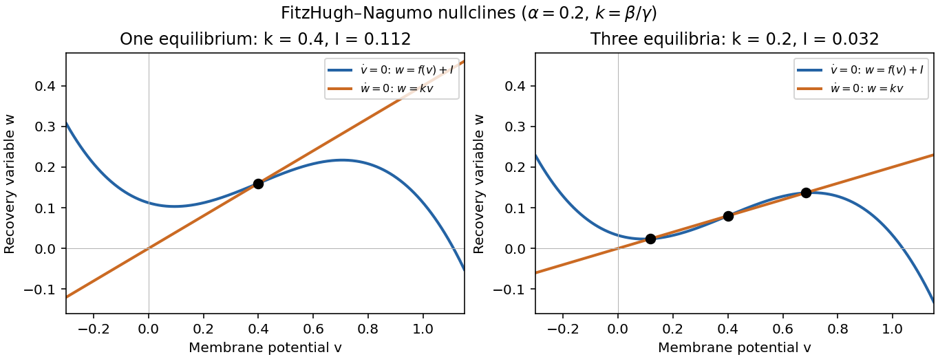
One and three intersections of the FitzHugh-Nagumo model nullclines
. Details. 
At an equilibrium , set . The Jacobian matrix, its trace and its determinant areThe eigenvalues and their discriminant areThus the complete local linear stability test isIn the last two cases, gives a node, while gives a focus; the sign of distinguishes inward and outward trajectories. At , a nonzero repeated eigenvalue gives a degenerate node. At the eigenvalues are purely imaginary, so linear stability analysis alone does not decide asymptotic stability; with the required crossing and nondegeneracy this is a Hopf bifurcation. At there is a zero eigenvalue, requiring a nonlinear test and generically marking the saddle-node bifurcation in the preceding answer.
For a unique simple equilibrium, , so it can be a sink equilibrium or a source equilibrium. The number of equilibria alone does not decide stability. If , the unique simple equilibrium is always a sink equilibrium. If , it can become a source equilibrium where . The same conclusion follows particularly simply if : the trace is negative at every nonsaddle equilibrium.
For three simple equilibria ordered by their coordinates, the middle one has and is a saddle equilibrium; the two outer ones have . When both outer equilibria are sink equilibria, each has an attracting neighborhood, giving bistability. In the usual two-basin portrait, the stable manifold of the saddle equilibrium separates their basins. Each branch of its unstable manifold initially leaves towards a different side; its eventual destination requires a global argument. If , both outer equilibria must be sink equilibria. If , either or both outer equilibria can instead be source equilibria; the same test applies separately to each. The three lower panels illustrate all three possibilities up to exchanging left and right.
The arrows in the phase plane follow directly from the nullclines: below the horizontal component points right, and above it left; below the vertical component points up, and above it down. Near a stable focus trajectories spiral inward; near an unstable focus they spiral outward. Near a saddle equilibrium they approach along its stable manifold and leave along its unstable manifold. These directions, together with the local tests, determine the sketches.
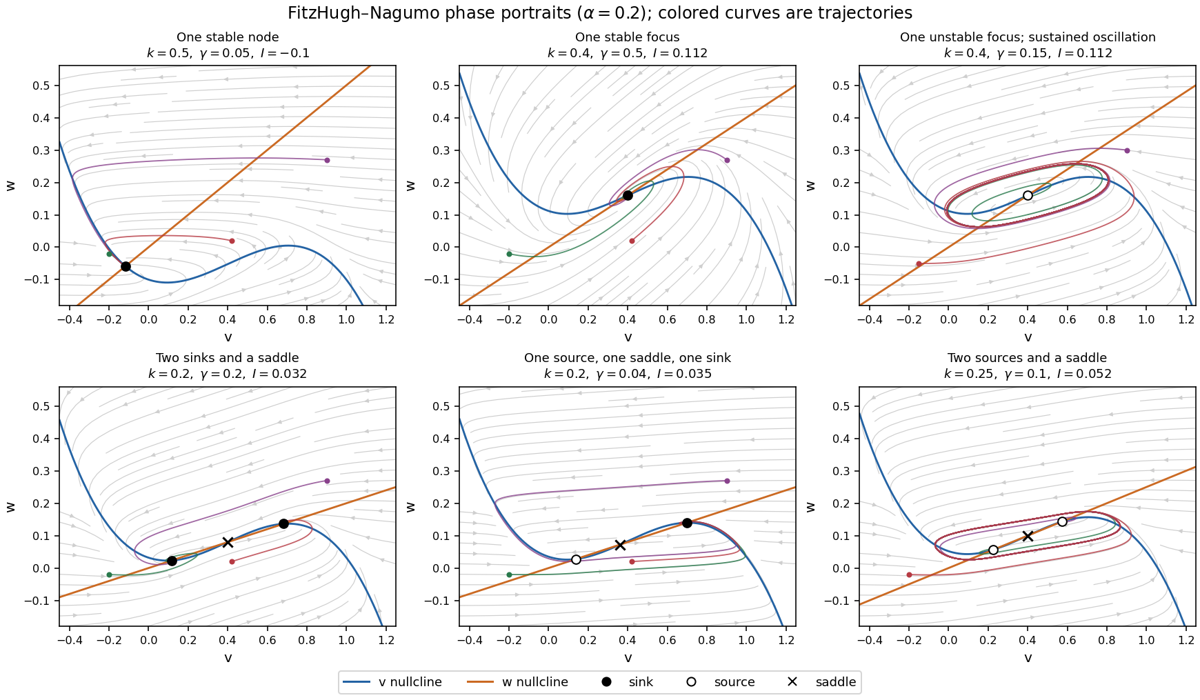
Phase portraits of the FitzHugh-Nagumo model with one or three equilibria, including changes of linear stability
. Details. 
There is also a useful global conclusion when the unique equilibrium is a source equilibrium. Withthe leading term in is , so sufficiently large ellipses are trapping regions. A small repelling neighborhood of the hyperbolic source equilibrium can be removed to form an invariant annulus. The Poincaré-Bendixson theorem then guarantees at least one periodic orbit in that annulus. The numerical sketch illustrates the resulting sustained oscillation; this argument does not assert uniqueness of a limit cycle. A stable equilibrium can instead represent a resting membrane potential, with perturbations producing damped relaxation; near a threshold, a sufficiently large perturbation can produce a large excursion before recovery. Global basin boundaries and coexistence of periodic orbits need more information than the number and local stability of equilibria.
Articles by others on the same topic
There are currently no matching articles.