The quantities are cell-cycle age densities: counts biological cells whose time since entering phase lies in . Here is time spent in the current phase, rather than time since birth. In this two-stage approximation to the cell cycle, a biological cell passes from G1 phase to G2 phase, then completes cell division and produces two daughters entering G1 phase.
The time derivative measures change at fixed phase age. The age derivative transports biological cells towards larger at unit speed, because . Thus each equation is an age-structured population equation. The nonnegative hazard function means that, conditional on still being in phase at age , the probability of leaving during the next is . Its product with is the loss from that phase-age class; it is not an additional death term.
The boundary condition at specifies the incoming flux. Every G1 phase exit contributes one entrant to G2 phase, whereas every G2 phase exit contributes two entrants to G1 phase. The initial conditions specify the phase-age composition at . Consequently integration over phase age gives the useful population balanceEach completed cell division increases the total number of biological cells by one.
The unit integrals of the profiles make the phase populations, and their normalized cell-cycle age densities. Assume the age tails vanish and the following integrals are finite. For a fixed profile define its mean exit hazard function byThese constants have units of inverse time. Integrating the age-structured population equations and using the boundary conditions givesThe incoming fluxes are and , soThe separable-profile closure for an age-structured population has a qualification: arbitrary age-dependent hazard functions do not give this constant-coefficient ordinary differential equation for arbitrary initial conditions. Without fixed , the effective exit rates are and can vary with time. Moreover, an exact positive separation of variables with both profiles fixed forces to be constant through the incoming fluxes, hence selects a common exponential mode. The displayed ordinary differential equation is the necessary integrated system for such profiles; it is also exact for arbitrary populations when both hazard functions are age independent.
Write for the population matrix and assume . Its characteristic polynomial isThe two eigenvalues have opposite signs. The dominant eigenvalue isand the other eigenvalue is . A positive eigenvector for satisfiesFor any nonzero nonnegative population vector in this constant-coefficient system, the coefficient of the positive eigenvector is positive: a positive left eigenvector annihilates the other eigenvector and has positive pairing with that population vector. Thus , with , and . The long-time leading term therefore obeys .
Substituting that exponential mode into the age-structured population equation givesDefine the phase-residence survival function and its discounted integral byThen the normalized cell-cycle age densities areSince integration of gives , this is equivalentlyThe constants must be consistent with both incoming fluxes. PutThe boundary conditions for amplitudes give and . Hence the Two-stage Euler-Lotka equation isIt determines directly from the hazard functions; the formula in terms of is not permission to choose those constants independently of the profiles. If each phase is eventually left with probability one, and decreases to zero, giving a unique positive root under the usual finite, non-instantaneous residence-time assumptions. More generally positive growth requires . Nonnegative hazard functions alone do not ensure it: if one phase has zero exit hazard function, growth cannot have the asserted positive exponent. Convergence of the complete age distribution to these profiles needs the usual mixing assumptions on phase-residence times; the two-dimensional eigenvalue calculation establishes the long-time claim for the fixed-profile system.
Because the hazard functions are constant, normalization gives and . The population characteristic polynomial factors asThusThese exponential distributions describe ages among currently present biological cells. Their rates differ from the phase-exit rates because exponential growth overrepresents younger entrants. The stable phase ratio is , so the G1 phase and G2 phase fractions approach and .
Increasing rescales all times by : the population undergoes faster exponential growth, its doubling time is , and the profile means and decrease. The phase fractions do not depend on . The population matrix has exact solutionso population-ratio transients decay relative to the growing term at rate . This exact population formula does not require initially stationary cell-cycle age densities.
Put . The nullclines of the space-clamped FitzHugh-Nagumo model areThe first nullcline is a downward-leading cubic polynomial, shifted vertically by ; the second nullcline is a line through the origin with slope . Their intersections satisfyWriting , differentiation givesIf , increases strictly, so there is exactly one equilibrium. If , is still strictly increasing, although its derivative vanishes at one point, so the equilibrium is again unique. If , defineHere has a local maximum at and a local minimum at ; thereforeAt either endpoint there are two distinct equilibria, one a double root. These are the saddle-node bifurcation boundaries omitted by the generic one-or-three wording. At and there is one triple root. This is the Cubic FitzHugh-Nagumo nullcline criterion.
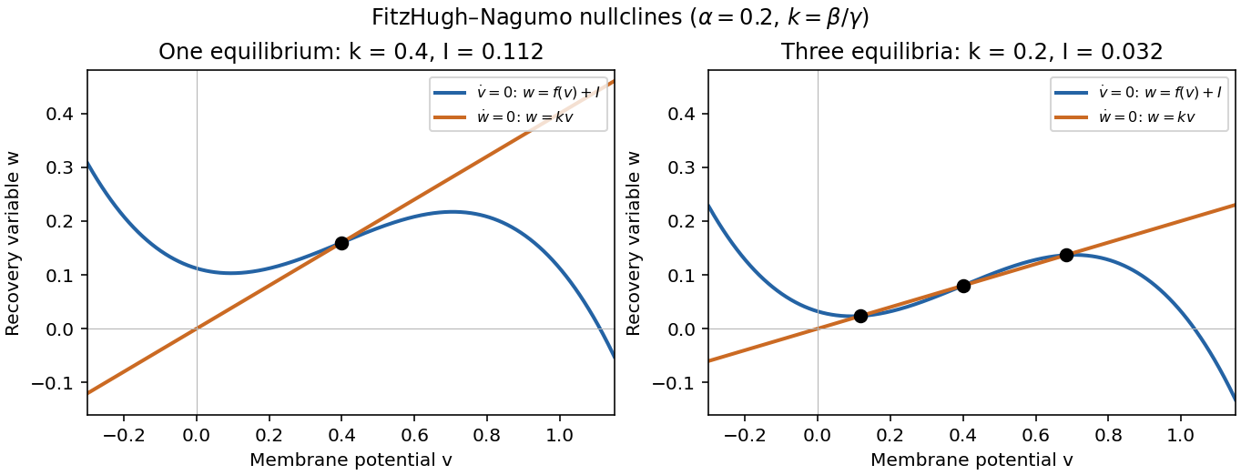
One and three intersections of the FitzHugh-Nagumo model nullclines
. Details. At an equilibrium , set . The Jacobian matrix, its trace and its determinant areThe eigenvalues and their discriminant areThus the complete local linear stability test isIn the last two cases, gives a node, while gives a focus; the sign of distinguishes inward and outward trajectories. At , a nonzero repeated eigenvalue gives a degenerate node. At the eigenvalues are purely imaginary, so linear stability analysis alone does not decide asymptotic stability; with the required crossing and nondegeneracy this is a Hopf bifurcation. At there is a zero eigenvalue, requiring a nonlinear test and generically marking the saddle-node bifurcation in the preceding answer.
For a unique simple equilibrium, , so it can be a sink equilibrium or a source equilibrium. The number of equilibria alone does not decide stability. If , the unique simple equilibrium is always a sink equilibrium. If , it can become a source equilibrium where . The same conclusion follows particularly simply if : the trace is negative at every nonsaddle equilibrium.
For three simple equilibria ordered by their coordinates, the middle one has and is a saddle equilibrium; the two outer ones have . When both outer equilibria are sink equilibria, each has an attracting neighborhood, giving bistability. In the usual two-basin portrait, the stable manifold of the saddle equilibrium separates their basins. Each branch of its unstable manifold initially leaves towards a different side; its eventual destination requires a global argument. If , both outer equilibria must be sink equilibria. If , either or both outer equilibria can instead be source equilibria; the same test applies separately to each. The three lower panels illustrate all three possibilities up to exchanging left and right.
The arrows in the phase plane follow directly from the nullclines: below the horizontal component points right, and above it left; below the vertical component points up, and above it down. Near a stable focus trajectories spiral inward; near an unstable focus they spiral outward. Near a saddle equilibrium they approach along its stable manifold and leave along its unstable manifold. These directions, together with the local tests, determine the sketches.
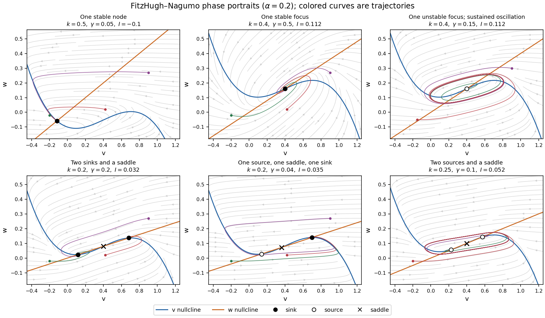
Phase portraits of the FitzHugh-Nagumo model with one or three equilibria, including changes of linear stability
. Details. There is also a useful global conclusion when the unique equilibrium is a source equilibrium. Withthe leading term in is , so sufficiently large ellipses are trapping regions. A small repelling neighborhood of the hyperbolic source equilibrium can be removed to form an invariant annulus. The Poincaré-Bendixson theorem then guarantees at least one periodic orbit in that annulus. The numerical sketch illustrates the resulting sustained oscillation; this argument does not assert uniqueness of a limit cycle. A stable equilibrium can instead represent a resting membrane potential, with perturbations producing damped relaxation; near a threshold, a sufficiently large perturbation can produce a large excursion before recovery. Global basin boundaries and coexistence of periodic orbits need more information than the number and local stability of equilibria.
There is a consistency issue in the printed model. If is imposed while retaining its evolution equation, then forces . Thus the full two-equation system has no nonconstant travelling wave with exactly constant . Its constant solution exists only when . The intended wave calculation must treat the recovery variable as externally frozen, leaving the scalar reaction-diffusion equationFor this frozen-recovery reduction, letThe cubic polynomial has a local minimum at and a local maximum at . Hence the conditiongives three distinct real roots of , withThe outer roots are stable for the scalar spatially uniform dynamics and the middle root is unstable. Seek a travelling wave , where . The travelling-wave reduction of a reaction-diffusion system givesLet and chooseIt has , andSubstitution leavesConsequently the frozen-recovery cubic front isReflection reverses the front and its speed. A nonzero speed requires ; equality gives a stationary front and is the Maxwell balance for a scalar reaction-diffusion front. Since the roots sum to , this stationary value is . For the simple admissible choice , the roots are andThis particular front moves when . At , other currents inside the displayed open interval give moving fronts.
The bacteria disperse by diffusion with coefficient . Their additional chemotaxis flux isIt points up the nutrient concentration gradient, and its negative spatial derivative enters the balance equation. The positive prevents singular sensitivity at zero nutrient concentration; increasing the background nutrient concentration reduces the drift response to a fixed gradient. The logistic growth equation term represents net reproduction with low-population growth rate and carrying capacity .
The nutrient undergoes diffusion with coefficient . Its production term is an increasing, bounded response to the bacteria, reaching half its maximum at . It has the algebraic form of a Hill equation with exponent two; the equation alone does not specify a molecular mechanism. The term removes nutrient at a rate proportional to both bacteria abundance and nutrient concentration.
The full fluxes areThe homogeneous Neumann boundary conditions make both fluxes vanish at the endpoints, so neither bacteria nor nutrient crosses the boundaries. The initial conditions specify their starting spatial distributions. This model includes nutrient production by bacteria, rather than a separate external supply term.
Use as the population scale, as the nutrient concentration scale, as the time scale, and as the length scale. The nondimensionalization isFor example, the chemotaxis term becomesDividing the population equation by and the nutrient equation by gives the requested system with the following six dimensionless quantities:The rescaled domain is , . Its boundary conditions and initial conditions are
For a spatially uniform steady state with nonzero bacteria abundance, forces . The nutrient balance then givesTo test spatially uniform linear stability, writeAt the positive equilibrium, the Jacobian matrix isIts eigenvalues are , both negative, so the positive equilibrium is asymptotically stable against spatially uniform perturbations. This remains true at , where a repeated eigenvalue may produce a decaying contribution. The printed stability claim must be understood in this spatially uniform sense: sufficiently strong chemotaxis can destabilize nonuniform perturbations, as the next answer shows.
Write , and defineThe first-order perturbation equations areThe homogeneous Neumann boundary conditions select Fourier modes proportional to , with squared wavenumber for . For a mode , the eigenvalue problem isIts trace is . Therefore a growing mode exists exactly when its determinant is negative. SetThe dispersion relation isThe constant mode has ; very short wavelengths also decay because . For a negative interval at positive , the upward-opening quadratic polynomial must have its minimum below zero at positive . This givesIn particular, is necessary, since otherwise and every coefficient of is positive. When , a locally increased population must increase net nutrient production, so attraction to that nutrient reinforces the population increase. This feedback must overcome both diffusion and local relaxation. The calculation is an instance of chemotactic instability with logistic growth and saturating production.
The displayed continuous-wavenumber inequality is necessary on the finite domain, but an allowed mode must actually lie in the unstable band:Equivalently, the exact discrete threshold isEquality gives a marginal zero eigenvalue rather than positive growth. At the unrestricted onset, , so . On the finite interval, Discrete Neumann mode selection first destabilizes the mode minimizing the discrete threshold; it need not attain exactly.
To predict the early form of a perturbation, use the larger growth eigenvalueFor , the square root is real. Choose maximizing among allowed modes with positive growth. The corresponding perturbation has wavelength in , or in . Its eigenvector satisfiesso bacteria and nutrient peaks initially coincide. A mode with larger has finer spatial structure. The two signs of are both allowed, exchanging peaks and troughs.
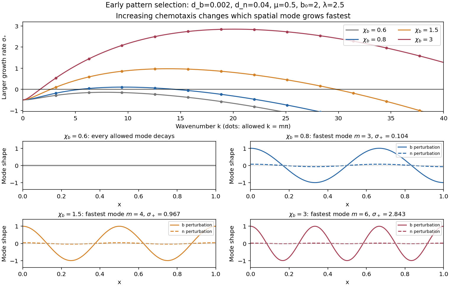


The illustration holds , , , and fixed, giving and , and varies . Crossing the discrete threshold makes a nonuniform Fourier mode grow; stronger chemotaxis widens the unstable band and can favor finer structure. Increasing either diffusion coefficient raises the threshold of each fixed mode. Varying can have a nonmonotone effect: with ,is maximal at , where . Additional production beyond that point weakens sensitivity enough to reduce this feedback. Changes in also change the allowed dimensional wavenumbers and all three scaled transport coefficients. These are predictions of linear stability analysis: eventual pattern amplitude, competition between growing modes and possible merging require the nonlinear system. The threshold is a necessary condition for spontaneous pattern growth from arbitrarily small perturbations, rather than a claim that every finite-amplitude nonuniform state is excluded below it.
Articles by others on the same topic
There are currently no matching articles.