Past exam of the mathematics course of the University of Cambridge / 2004 / ia / Paper 2 / Section I

For a straight-line solution $y=mx$, substitution into the differential equation gives $m=(1-2m)/(2+m)$. Thus $m^2+4m-1=0$, and the two possible slopes areThese straight lines solve the differential equation on either side of the origin. At the origin itself the right-hand side is undefined.

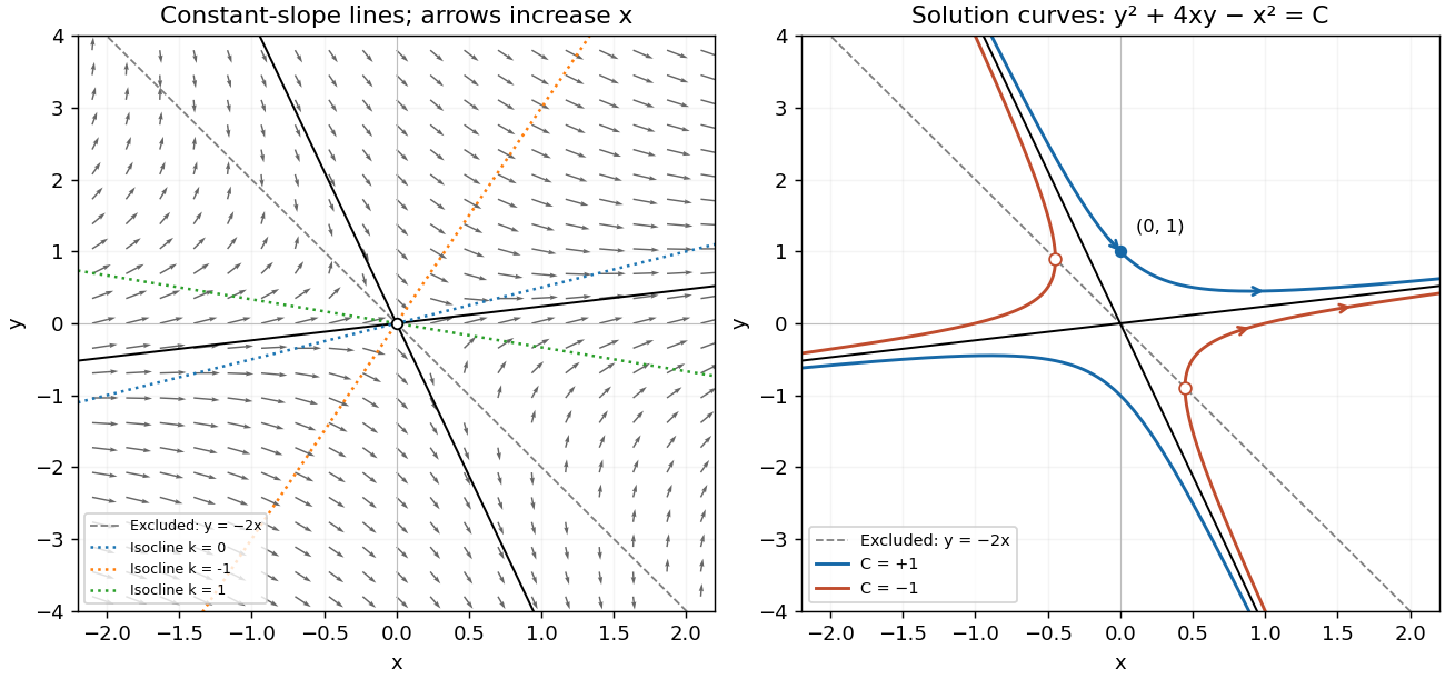
An isocline of slope $k$ has equation $(1-2k)x-(2+k)y=0$. For $k\ne -2$ it is the straight line $y=(1-2k)x/(2+k)$; for $k=-2$ it is $x=0$, excluding the origin. In particular, $y=x/2$ is the zero-slope isocline. The line $y=-2x$ is excluded from the domain of the differential equation; slopes tend to infinity on approaching it. Draw the flow vectors proportional to $(1,(x-2y)/(2x+y))$, with positive horizontal component. This specifies orientation by increasing $x$, rather than by an auxiliary time variable.

To integrate, put $y=xu$ where $x\ne 0$. ThenThe left-hand integral is $-\frac{1}{2}\log |1-4u-u^2|$, so the nonconstant-$u$ solutions have the first integralThe constant-$u$ solutions omitted by separation are exactly the two straight lines already found, corresponding to $C=0$. Alternatively, differentiating this first integral gives $(2y+4x)y^{\prime }+4y-2x=0$, which recovers the original differential equation wherever $2x+y\ne 0$ and also verifies continuation through $x=0$ when $y\ne 0$.

The first integral describes hyperbolas with the two straight-line solutions as asymptotes. For $C=1$, the upper branch crosses the vertical axis at $(0,1)$ and exists for every real $x$. For $C=-1$, each branch is confined to $|x|\ge 1/\sqrt{5}$ and reaches a vertical tangent on the excluded line $y=-2x$; the corresponding classical solution intervals exclude those endpoints. These give the two distinct types of curves requested in the sketch.

The initial condition selects $C=1$ and the upper branch, henceHere $2x+y=\sqrt{5x^2+1}>0$, so this really is a global solution of the initial value problem, and $y^{\prime }(0)=-2$ agrees with the right-hand side.

Write $y=e^{-px}v$. Direct differentiation givesThe homogeneous linear differential equation therefore has $v=A+Bx$. A linearly independent pair of solutions isTheir Wronskian is $e^{-2px}$, which never vanishes; the argument also includes $p=0$.

For the inhomogeneous linear differential equation, the same substitution gives $v^{\prime \prime }=1$. Since $y(0)=0$ implies $v(0)=0$, and $y^{\prime }(0)=0$ then implies $v^{\prime }(0)=0$, integration gives $v=x^2/2$. Thus the required solution of the initial value problem is

For random variables with finite second moments, their covariance isThe Cauchy-Schwarz inequality ensures the product is integrable under this hypothesis. More generally the definition works whenever the displayed expectations exist. Assertions about arbitrary random variables below are understood on this domain: without suitable moments a covariance need not be defined at all.

Linearity of expectation gives $\mathbb{E}(X+Y)=\mathbb{E}X+\mathbb{E}Y$. Expand the centered product and use linearity of expectation again:Thus the assertion is true whenever the covariances are defined. Neither independence nor identical distributions are required.

The covariance is symmetric, because multiplication of real random variables is commutative. Expanding with the bilinearity just proved givesIdentical probability distributions imply equal second moments and equal means, hence equal variances. Therefore the assertion is true, withThe cancellation shows exactly why no assumption of independence is needed.

A probability density function must integrate to one. ThereforeThe first two moments areConsequently the mean and variance are