Past exam of the mathematics course of the University of Cambridge / 2004 / iii / Paper 39 / 3

Only the copies inherited through the two related parents can share recent identity by descent; the other parental contributions come from unrelated founders in a pedigree. The related parents are full siblings. Their transmitted copies trace to the same shared grandparent with probability $1/2$, and then to the same copy of that grandparent with probability $1/2$. Thus the first-cousin identity-by-descent probabilities areTo compute the kinship coefficient, one random copy from each cousin selects those potentially shared contributions with probability $1/4$. Hence

An offspring is autozygous precisely when its two transmitted parental copies are identical by descent. Therefore its inbreeding coefficient equals the parental kinship coefficient, giving the first-cousin inbreeding coefficient

Use identity-by-descent sharing of inbred full siblings, with $J$ the maximum number of copies that can be paired across the children as identical by descent. If two copies within one child have the same ancestral origin, they still count as two copies when both can be paired.

With probability $3/4$ the cousin parents share no ancestral copy. Conditional on this event, their children have ordinary Mendelian IBD sharing of full siblings, namely $(1/4,1/2,1/4)$. With probability $1/4$, the parental copies can be labelled $(A,B)$ and $(A,C)$, with $A,B,C$ distinct ancestral origins. Each child independently receives one of $AA,AB,AC,BC$, with probability $1/4$ each. Among the sixteen ordered child pairs, $AA$ paired with $BC$ in either order gives $J=0$; four equal genotype-origin pairs give $J=2$; the remaining ten give $J=1$. The mixture isThese are inbred children, so the three sharing probabilities do not retain all within-child identities. The full Jacquard identity coefficients are $(1,0,2,1,2,1,15,30,12)/64$. In particular, their kinship coefficient is $9/32$; applying the outbred formula $(P(J=1)+2P(J=2))/4$ here would be incorrect.

Label the full siblings at the bottom $X,Y$ and their cousin parents $F,M$. Let $F$ have parents $A,B$ and $M$ parents $C,D$, where $A,C$ are siblings with parents $U,V$. Include the other great-grandparents as $P,Q$, parents of $B$, and $R,S$, parents of $D$. This gives fourteen people, with six independent founders in a pedigree $U,V,P,Q,R,S$.

The pedigree graphical model has the following Directed acyclic graph, with both members of each parent pair pointing to every listed child:Let $f(g)$ be the founder genotype law under Hardy-Weinberg equilibrium, and let $t(g\mid h,k)$ be the Mendelian segregation kernel. The joint probability of all genotypes isFor a biallelic locus with allele-1 frequency $p$, $f(11)=p^2$, $f(12)=2p(1-p)$ and $f(22)=(1-p{)}^2$. The kernel $t$ assigns probability $1/4$ to each labelled pair of parental transmissions and adds these probabilities when they produce the same unordered genotype. Summing this Bayesian network factorization over unobserved genotypes gives their marginal distribution or a pedigree likelihood.

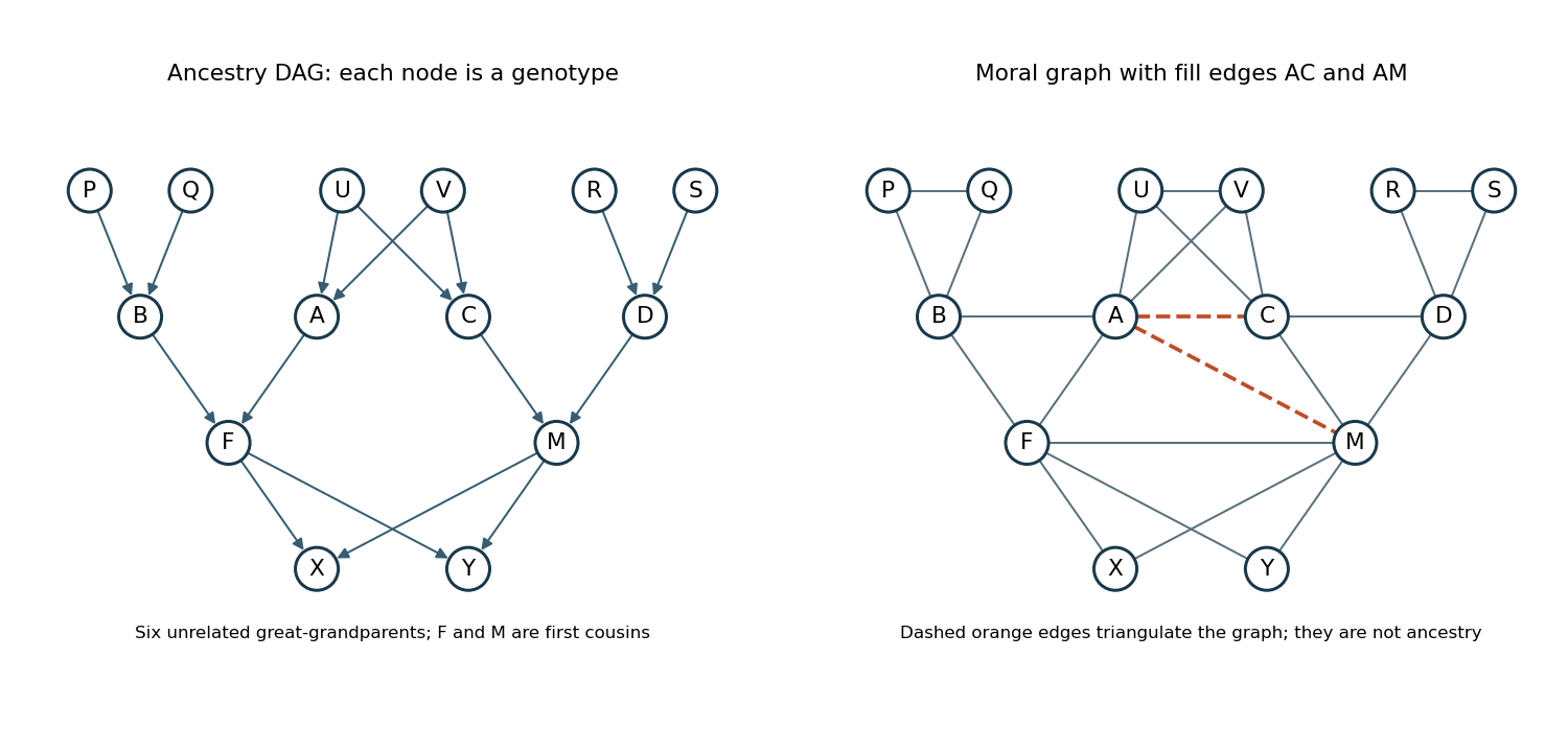
For the undirected representation of the pedigree graphical model, take the moral graph: remove arrowheads from all parent-child edges and join coparents. The added coparent edges areEvery Mendelian segregation factor involves a child and its two parents, so its variables form a clique in this graph. The product in the previous part is thus an undirected factorization. A separation of variables by a conditioning set in this graph implies the corresponding conditional independence.

This is a valid conditional independence graph representation of the joint genotype law. It need not be its minimal representation without a faithfulness of a directed acyclic graph assumption: some inheritance probabilities are zero, and special parameter choices can yield additional independences. It also differs from a graph of unconditioned correlations, since full siblings remain correlated through their parents when the parental genotypes are not conditioned on.

A valid triangulation of an undirected graph adds exactly the two fill edgesTo verify it, eliminate the vertices in the order $P,Q,R,S,X,Y,B,D,F,M,A,C,U,V$. The first eight eliminations have neighboring vertices already joined. When $F$ is eliminated, its remaining neighbors are $A,M$, so add $AM$. When $M$ is eliminated, its remaining neighbors are $A,C$, so add $AC$. The remaining $A,C,U,V$ form a clique.

Thus this order is a perfect elimination ordering of the completed graph, which is a chordal graph. The fill edges are computational devices for genotype elimination; they do not add parent-child relationships to the pedigree.

The nine maximal cliques of this triangulation areEvery other nonempty clique is a subset of one of these. One junction tree, listing its separators after the edges, isEach variable appears in a connected subtree, verifying the running intersection property. For example, the cliques containing $M$ are $K_1,K_2,K_4,K_5,K_6$, and their connecting paths contain $M$ throughout.

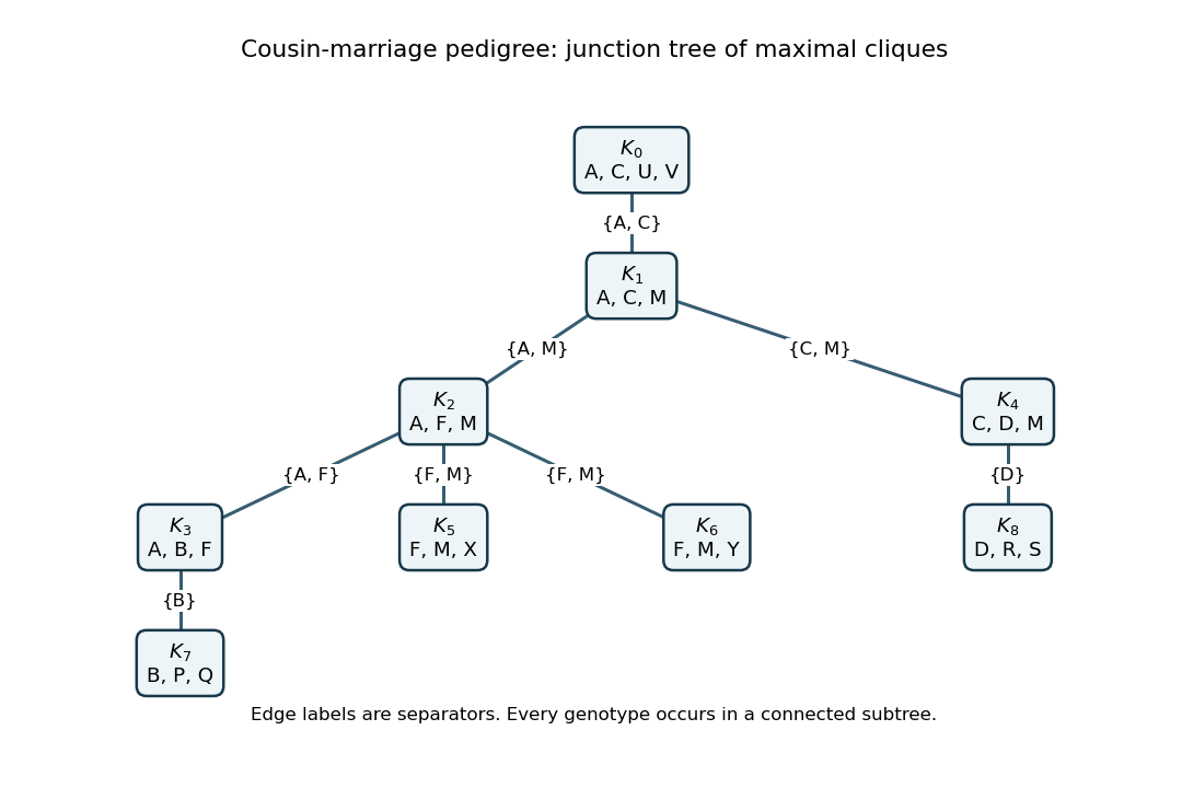
The junction tree algorithm assigns every founder factor and every child-with-parents factor to one containing clique, and multiplies any observation or penetrance factors there. The junction-tree sum-product message from clique $i$ to clique $j$ sums out $C_i\setminus (C_i\cap C_j)$ after multiplying the local potential and all incoming messages except $j$'s. An inward pass sums the joint probability or pedigree likelihood; a subsequent outward pass gives each person's posterior genotype probabilities. This is the same variable-elimination principle as the Elston-Stewart algorithm, organized to handle the pedigree loop. Its largest clique has four genotype variables, much smaller than summing naively over fourteen at once.