Past exam of the mathematics course of the University of Cambridge / 2004 / iii / Paper 39 (Statistical and Population Genetics)

During the epoch with $j$ ancestral lineages, Kingman's coalescent has waiting time $T_j\sim \mathrm{Exp}((\genfrac{}{}{0ex}{}{j}{2}))$. In the stated time units, each lineage accumulates mutations at rate $Nu=\theta /2$, so the mutation count on a neutral coalescent tree decomposes asThe law of total expectation and the mean of an exponential distribution give $\mathbb{E}{Y}_j=(j\theta /2)/\left(\genfrac{}{}{0ex}{}{j}{2}\right)=\theta /(j-1)$. ThereforeThis calculation counts mutation events. Equating the count with observed segregating sites additionally uses the infinite sites mutation model.

Apply the law of total variance to each epoch. The Poisson distribution has equal conditional mean and variance, while $\mathrm{Var}(T_j)={\left(\genfrac{}{}{0ex}{}{j}{2}\right)}^{-2}$. HenceThe independent mutation counts in coalescent epochs permit variance additivity for independent random variables. ThusThe first term is conditional Poisson distribution variation; the second comes from the random lengths of the ancestral tree. These are the moments of the mutation count on a neutral coalescent tree.

The Watterson estimator isThe expectation above makes it an unbiased estimator. Its variance, given by the variance of the Watterson estimator, isIndeed, the harmonic sum satisfies $H_{n-1}\sim \log n$ and $H_{n-1}^{(2)}$ stays bounded. This proves mean-square convergence; the Chebyshev inequality then shows that it is a consistent estimator, since $P(|\hat{\theta }-\theta |>\epsilon )\le \mathrm{Var}(\hat{\theta })/{\epsilon }^2\to 0$.

Conditioning on the epoch length gives the probability generating functionThe Laplace transform of an exponential distribution then yieldsThis is the geometric mutation count in a coalescent epoch. With the zero-based geometric distribution convention,At $\theta =0$, this reduces to $Y_j=0$ almost surely.

For fixed $\theta >0$, use the Lyapunov condition for the independent centered epoch counts $Z_i=Y_{i+1}-\theta /i$. Their total variance is $s_n^2=\theta H_{n-1}+{\theta }^2{H}_{n-1}^{(2)}\sim \theta \log n$.

Write ${\mu }_i=\theta /i$. Differentiating the geometric distribution probability generating function gives $\mathbb{E}[Y_{i+1}^3]={\mu }_i+6{\mu }_i^2+6{\mu }_i^3$. Since $|Y_{i+1}-{\mu }_i{|}^3\le 4Y_{i+1}^3+4{\mu }_i^3$, the sum of the centered absolute third moments is $O(\log n)$. ConsequentlyThe Lindeberg-Feller central limit theorem applies through the Lyapunov condition, giving $(S-\theta H_{n-1})/s_n\stackrel{d}{\to }N(0,1)$. Now $\sqrt{\log n}{s}_n/H_{n-1}\to \sqrt{\theta }$, so the Slutsky theorem proves the asymptotic normality of the Watterson estimator:The limiting variance is $\theta$. When $\theta =0$, every count vanishes and the limiting law is the point mass at zero.

The asymptotic normality of the Watterson estimator gives approximate standard error $\sqrt{\theta /\log n}$. Thus precision at a fixed nonrecombining locus improves only logarithmically with sample size. To halve the asymptotic standard error, one needs $\log n^{\prime }\simeq 4\log n$, or roughly $n^{\prime }=n^4$, rather than four times as many sampled chromosomes.

For large samples and positive $\hat{\theta }$, a plug-in normal approximation gives $\hat{\theta }\pm 1.96\sqrt{\hat{\theta }/\log n}$ as an approximate 95% confidence interval. At low mutation counts it can perform poorly or give a negative endpoint; the exact count model is then preferable. Multiple independent, comparable loci can provide additional independent information, whereas tightly linked chromosomes still share the random ancestry at one locus. Genetic recombination, nonneutral evolution and changing population size require corresponding changes to the model.

Linkage disequilibrium means that alleles at different genetic loci are associated in population haplotypes. For two biallelic loci,The first quantity measures departure from independent allele frequencies; the second is the squared allelic correlation. Standardized linkage disequilibrium $D^{\prime }$ instead compares $D$ to its possible range at the given frequencies. High $|D^{\prime }|$ can coexist with low $r^2$, so it need not make one genetic marker a good predictor of another. Genetic linkage is a different notion: it describes within-family transmission and the recombination fraction.

The chromosome-21 study of Patil and colleagues, Science 2001 found consecutive single-nucleotide polymorphisms organized into regions with comparatively few common haplotypes; typically three haplotypes accounted for over 80% of the sampled chromosomes within a block. Such haplotype blocks can be represented efficiently by tag SNPs. Strong association within blocks and weaker association across boundaries give a useful description, though block boundaries depend on allele frequencies, population history, sampling and the operational definition of a block. They do not divide chromosomes into regions where genetic recombination is respectively impossible and certain.

The ancestry explanation uses an ancestral recombination graph. Going backwards, ancestral lineages coalesce, while a genetic recombination event splits one lineage's ancestral material into contributions from two parents. At a fixed genomic position, retaining only its ancestry gives a phylogenetic tree with the appropriate coalescent law. Nearby positions often retain much of the same tree; mutations on shared branches then produce correlated allele states. Breakpoints can change the local tree, weakening that shared history.

Under a simple random-mating two-locus model, linkage-disequilibrium decay under recombination gives $D_{t+1}=(1-r)D_t$. Actual populations also undergo genetic drift, population bottlenecks, mutation and migration, which can create or preserve association. Recombination rates themselves vary along chromosomes: McVean and colleagues, Science 2004 inferred strong local variation from sequence data. These observations motivate an ancestry model with spatially varying recombination, rather than treating physical distance as the only determinant of linkage disequilibrium.

For fine mapping, a typed genetic marker can show genetic association because it is correlated with a nearby causal genetic variant. Linkage-disequilibrium marker tagging makes a sparse first-stage scan possible, but several variants in one block can produce nearly indistinguishable association patterns. Historical recombination and diverse local genealogies can narrow the interval when denser genotyping is available.

An ancestral recombination graph turns that intuition into a likelihood calculation. One can place a proposed disease-origin event on a local ancestral branch and integrate over possible graphs, mutation histories and unobserved haplotypes. The local phylogenetic tree then relates disease-bearing chromosomes and predicts which markers should remain associated. In a Bayesian inference, uncertainty in ancestry, mutation location and demographic parameters enters the posterior distribution rather than being replaced by one guessed tree. Whole-graph inference is computationally demanding, and approximate or pairwise methods often supply practical estimates.

The useful distinction is between finding an associated region and identifying its causal variant. Strong linkage disequilibrium improves marker coverage but can limit resolution inside the associated region. Population stratification, ascertainment, rare variants and misspecified population history can also mislead an association analysis. Combining fine mapping with independent biological evidence is therefore stronger than interpreting an association peak as proof of causation.

Only the copies inherited through the two related parents can share recent identity by descent; the other parental contributions come from unrelated founders in a pedigree. The related parents are full siblings. Their transmitted copies trace to the same shared grandparent with probability $1/2$, and then to the same copy of that grandparent with probability $1/2$. Thus the first-cousin identity-by-descent probabilities areTo compute the kinship coefficient, one random copy from each cousin selects those potentially shared contributions with probability $1/4$. Hence

An offspring is autozygous precisely when its two transmitted parental copies are identical by descent. Therefore its inbreeding coefficient equals the parental kinship coefficient, giving the first-cousin inbreeding coefficient

Use identity-by-descent sharing of inbred full siblings, with $J$ the maximum number of copies that can be paired across the children as identical by descent. If two copies within one child have the same ancestral origin, they still count as two copies when both can be paired.

With probability $3/4$ the cousin parents share no ancestral copy. Conditional on this event, their children have ordinary Mendelian IBD sharing of full siblings, namely $(1/4,1/2,1/4)$. With probability $1/4$, the parental copies can be labelled $(A,B)$ and $(A,C)$, with $A,B,C$ distinct ancestral origins. Each child independently receives one of $AA,AB,AC,BC$, with probability $1/4$ each. Among the sixteen ordered child pairs, $AA$ paired with $BC$ in either order gives $J=0$; four equal genotype-origin pairs give $J=2$; the remaining ten give $J=1$. The mixture isThese are inbred children, so the three sharing probabilities do not retain all within-child identities. The full Jacquard identity coefficients are $(1,0,2,1,2,1,15,30,12)/64$. In particular, their kinship coefficient is $9/32$; applying the outbred formula $(P(J=1)+2P(J=2))/4$ here would be incorrect.

Label the full siblings at the bottom $X,Y$ and their cousin parents $F,M$. Let $F$ have parents $A,B$ and $M$ parents $C,D$, where $A,C$ are siblings with parents $U,V$. Include the other great-grandparents as $P,Q$, parents of $B$, and $R,S$, parents of $D$. This gives fourteen people, with six independent founders in a pedigree $U,V,P,Q,R,S$.

The pedigree graphical model has the following Directed acyclic graph, with both members of each parent pair pointing to every listed child:Let $f(g)$ be the founder genotype law under Hardy-Weinberg equilibrium, and let $t(g\mid h,k)$ be the Mendelian segregation kernel. The joint probability of all genotypes isFor a biallelic locus with allele-1 frequency $p$, $f(11)=p^2$, $f(12)=2p(1-p)$ and $f(22)=(1-p{)}^2$. The kernel $t$ assigns probability $1/4$ to each labelled pair of parental transmissions and adds these probabilities when they produce the same unordered genotype. Summing this Bayesian network factorization over unobserved genotypes gives their marginal distribution or a pedigree likelihood.

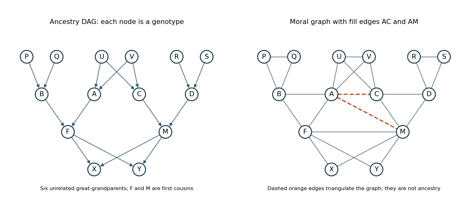
For the undirected representation of the pedigree graphical model, take the moral graph: remove arrowheads from all parent-child edges and join coparents. The added coparent edges areEvery Mendelian segregation factor involves a child and its two parents, so its variables form a clique in this graph. The product in the previous part is thus an undirected factorization. A separation of variables by a conditioning set in this graph implies the corresponding conditional independence.

This is a valid conditional independence graph representation of the joint genotype law. It need not be its minimal representation without a faithfulness of a directed acyclic graph assumption: some inheritance probabilities are zero, and special parameter choices can yield additional independences. It also differs from a graph of unconditioned correlations, since full siblings remain correlated through their parents when the parental genotypes are not conditioned on.

A valid triangulation of an undirected graph adds exactly the two fill edgesTo verify it, eliminate the vertices in the order $P,Q,R,S,X,Y,B,D,F,M,A,C,U,V$. The first eight eliminations have neighboring vertices already joined. When $F$ is eliminated, its remaining neighbors are $A,M$, so add $AM$. When $M$ is eliminated, its remaining neighbors are $A,C$, so add $AC$. The remaining $A,C,U,V$ form a clique.

Thus this order is a perfect elimination ordering of the completed graph, which is a chordal graph. The fill edges are computational devices for genotype elimination; they do not add parent-child relationships to the pedigree.

The nine maximal cliques of this triangulation areEvery other nonempty clique is a subset of one of these. One junction tree, listing its separators after the edges, isEach variable appears in a connected subtree, verifying the running intersection property. For example, the cliques containing $M$ are $K_1,K_2,K_4,K_5,K_6$, and their connecting paths contain $M$ throughout.

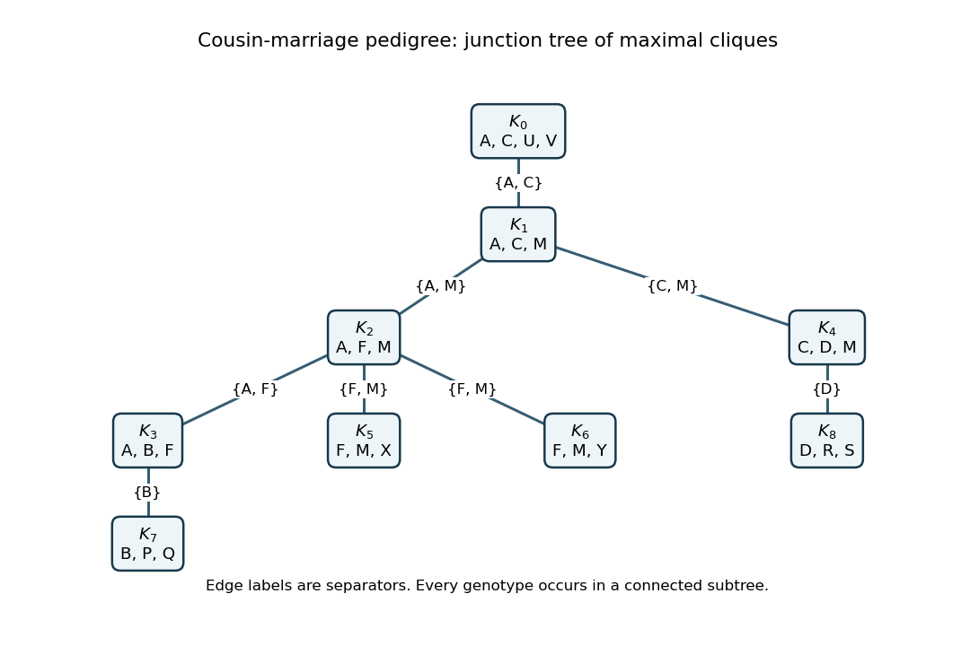
The junction tree algorithm assigns every founder factor and every child-with-parents factor to one containing clique, and multiplies any observation or penetrance factors there. The junction-tree sum-product message from clique $i$ to clique $j$ sums out $C_i\setminus (C_i\cap C_j)$ after multiplying the local potential and all incoming messages except $j$'s. An inward pass sums the joint probability or pedigree likelihood; a subsequent outward pass gives each person's posterior genotype probabilities. This is the same variable-elimination principle as the Elston-Stewart algorithm, organized to handle the pedigree loop. Its largest clique has four genotype variables, much smaller than summing naively over fourteen at once.

Count one transmitted/untransmitted allele pair per observable parent. A homozygous parent contributes to $a$ or $d$; a heterozygous parent contributes to $b$ or $c$. When two heterozygotes have a heterozygous child, the parent-specific origin is ambiguous, but the combined contribution is unambiguously one to $b$ and one to $c$.

The derived contributions, ordered as $(a,b,c,d)$, areIn family 7, the observed father's transmission cannot be determined from the heterozygous child without the mother's genotype. In family 10, the homozygous child reveals the father's allele-1 transmission, but not the missing mother's complete transmitted/untransmitted pair.

Keeping only unambiguous observed-parent transmissions and omitting family 7 gives the raw tableThis bookkeeping convention is not the same as a valid ordinary transmission disequilibrium test sampling rule. Incomplete-trio transmission-selection bias arises if only homozygous children make a missing-parent family usable. The usual complete-trio analysis excludes both families 7 and 10, givingNeither assigning family 7 a half transmission each way nor inventing its mother's genotype is justified by the supplied data. A method using all twelve families must model or validly condition on the missing information.

The transmission disequilibrium test is the paired McNemar test statistic $(b-c{)}^2/(b+c)$. From the raw unambiguous-transmission table,The formal one-degree-of-freedom chi-squared distribution approximation gives $p\simeq 0.071$, so the calculation does not reject at 5%. Its ordinary null calibration would require a valid missing-parent inclusion rule; the raw arithmetic alone does not establish one.

Using the complete-trio table gives ${\chi }_{\mathrm{TDT}}^2=36/14=18/7\simeq 2.571$, with $p\simeq 0.109$. It also does not reject. Homozygous-parent transmissions in $a,d$ supply no discordant contrast for this test.

The unmatched haplotype-relative-risk counts satisfy $w=a+b$, $x=c+d$, $y=a+c$ and $z=b+d$. For the raw table this givesThe Pearson chi-squared test of independence in this two-by-two table has statisticThus the unmatched calculation gives nominal evidence at 5%, with $p\simeq 0.030$. It differs from the transmission disequilibrium test because it uses an unmatched table, and it also inherits the missing-parent selection issue from the raw counts.

For the ten complete trios, $(w,x,y,z)=(12,8,6,14)$, giving odds ratio $7/2$ and the unmatched Pearson chi-squared test of independence statistic $40/11\simeq 3.636$, with $p\simeq 0.057$. That calculation does not reject at 5%. The nominal significance from the raw table therefore should not be presented as a robust association conclusion without a justified model for incomplete families and the unmatched-table assumptions.

The disease-ascertained transmission probability follows directly from Bayes' theorem. Assume that, given the child's genotype $g$, its disease probability is a common baseline penetrance times the genotype relative risk $R_g$, with no additional dependence on the parental genotypes. Write $q_g=P(g\mid g_f,g_m)$ for the Mendelian segregation probability. ThenThere are four equally likely labelled parental transmission outcomes. For one specified outcome $t$, this becomes $P(t\mid g_f,g_m,D)=R_{g(t)}/{\sum }_{t^{\prime }}{R}_{g(t^{\prime })}$, which is the four-outcome interpretation of the displayed formula.

For an unordered child genotype, let $m_g$ be the number of those outcomes producing it. Its probability is insteadFor example, two heterozygous parents have multiplicities $(1,2,1)$ for $11,12,22$. A heterozygous child therefore has probability $2R_{12}/(R_{11}+2R_{12}+R_{22})$. The four possible outcomes must be counted with multiplicity; treating their unordered genotypes as four distinct equally likely values would be incorrect.

Let $A=R_{11}+2R_{12}+R_{22}$. Among the ten complete trios, six have two heterozygous parents: three have child $11$, two have child $12$ and one has child $22$. Their conditional likelihood contribution isTwo more trios have a heterozygous parent and a $22$ parent, with child $12$ in each; they contribute $[R_{12}/(R_{12}+R_{22}){]}^2$. The remaining two parent pairs can produce only child $12$, so their conditional probabilities are one. Multiplying givesThe factor $4$ does not depend on the genotype relative risks, so the conventional proportional likelihood function isThis is the expression in the original PDF, up to the parameter-independent constant. Its last denominator is $R_{12}+R_{22}$; the converted TeX's $R_{11}+R_{22}$ is a transcription error. The factor $4$ in the exact probability comes from the two heterozygous children of two heterozygous parents, each of which has two labelled transmission routes.