Set . Equilibria satisfy , and their scalar linear eigenvalue isIt vanishes only at or . Substitution in the equilibrium relation gives the three nonhyperbolic parameter-state pointsThe branches with and are stable, while is unstable. For there are three equilibria; beyond the two outer saddle-node bifurcations there is just the positive stable one. At there is also the distinct stable equilibrium .
Near the crossing, use the smooth coordinate , whose derivative is positive near zero. The equation becomes with . A positive time rescaling removes , and the parameter-dependent state shift givesThus the crossing at is a transcritical bifurcation, with parameter . The two smooth branches exchange dynamical stability; labeling the stable branch by instead would obscure that exchange. The parameter-dependent coordinate shift in a transcritical bifurcation explains why the original coordinate need not display a branch identically equal to zero.
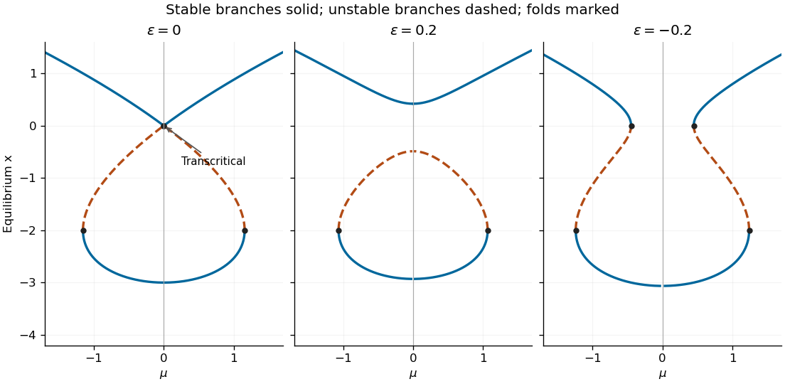
Scalar equilibrium diagrams before and after positive and negative unfolding, with stable branches solid and unstable branches dashed
. Details. 
Write . The entire unfolded diagram is obtained from , with the same dynamical stability sign as before. A saddle-node bifurcation at requires , while a saddle-node bifurcation at requires .
For , the crossing separates into a positive stable branch and a negative unstable branch, with no saddle-node bifurcation near . Three equilibria exist for , and the two negative branches annihilate at the outer saddle-node bifurcations . Outside that interval only the positive stable equilibrium remains. If , the diagram has just that one branch everywhere; equality is the limiting saddle-node bifurcation contact at .
For , let . Two inner saddle-node bifurcations occur at , and two outer saddle-node bifurcations at . For there is a single stable equilibrium below ; for there are three equilibria with stable–unstable–stable ordering; outside the outer saddle-node bifurcations only the positive stable equilibrium remains. The preceding figure shows representative small unfoldings. In particular this unrestricted perturbation destroys the exact transcritical bifurcation crossing.
Put . The planar vector field and its equilibrium eigenvalue data areFor a nonzero equilibrium, use to rewrite the determinant as . These formulas determine the local bifurcations of the imperfect soft Duffing-van der Pol oscillator directly.
When , the origin is a saddle equilibrium for and has determinant for ; the two equilibria are saddle equilibria. They meet the origin in a symmetry-protected pitchfork bifurcation at for . At the origin undergoes a supercritical Hopf bifurcation. To determine criticality, take : averaging gives , so the stable small limit cycle has .
The potential energy of the conservative part and the exact energy balance areAt zero imperfection the stable limit cycle grows to a heteroclinic cycle connecting the two outer saddle equilibria. Near the double-zero point its leading connection curve can be calculated, rather than inferred just from symmetry. In the Hamiltonian system limit the heteroclinic orbit is , andThe weak-damping persistence condition is therefore , not an exact formula at order-one parameters.
Now take ; negative imperfection reflects the phase portrait. The pitchfork bifurcation unfolds into a transcritical bifurcation crossing at and a saddle-node bifurcation at . The latter occurs at . Between those values the origin and are saddle equilibria, while lies in and is a sink or source according to the trace. At , exchanges its saddle equilibrium/non-saddle character with the origin. The double-zero points are now at and .
The original Hopf bifurcation line remains, still supercritical. A second Hopf bifurcation curve occurs on the intermediate nonzero equilibrium:It is important not to assign the same criticality to its entire length. Write , so . Around that center the restoring quadratic coefficient is , the damping linear coefficient is , and . The Hopf criticality for an asymmetric Lienard center calculation gives cubic amplitude coefficientHence it is supercritical for and subcritical for , with a generalized Hopf bifurcation point at . Higher-order terms are needed exactly there. For small imperfection the leading quintic coefficient is positive: writing and using the coordinate that normalizes the potential energy, , with and , the coefficient of in at vanishing cubic coefficient is . Weak-damping averaging therefore supplies the nearby saddle-node bifurcation of stable and unstable limit cycles in the generalized Hopf bifurcation unfolding. None of these small features intersects either requested parameter line.
Globally, the two saddle equilibrium barriers are no longer equal. Their leading energy difference is . The two one-way connections consequently separate; matching their energy differences with the connection integral givesThese weak-damping heteroclinic splitting of a tilted quartic oscillator formulas apply for small with . Between the separated connection curves, the central stable limit cycle terminates in a homoclinic orbit to the lower-barrier saddle equilibrium, for positive imperfection. The simultaneous symmetric heteroclinic-cycle destruction is therefore replaced by two basin-changing one-way connections and a distinct homoclinic orbit loss of the limit cycle. Its period diverges at that loss.
Along , decrease from above one. The sequence is supercritical Hopf bifurcation at ; first heteroclinic orbit; homoclinic orbit loss of the stable limit cycle; second heteroclinic orbit; transcritical bifurcation crossing at zero; saddle-node bifurcation at . The connection locations are global, not obtained by treating the Melnikov approximation as exact. For illustration, direct stable/unstable manifold matching at places them at approximately , respectively. The diagram below gives the qualitative ordering without prescribing those example values for arbitrary imperfection.
Along , the sequence is simply transcritical bifurcation crossing at zero, followed by saddle-node bifurcation at . Before the latter, in the relevant region, so decreases strictly on nonstationary trajectories and there is no periodic orbit or saddle equilibrium loop. After it only a saddle equilibrium remains, which cannot be enclosed by a periodic orbit by the Poincare-index obstruction to a periodic orbit. The origin does not undergo a Hopf bifurcation at , since its determinant there is negative.
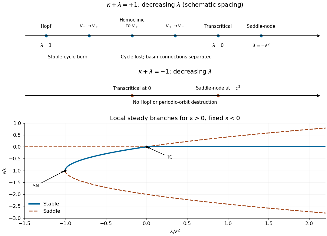
Bifurcation sequences along the two diagonal parameter lines after a small positive reflection-symmetry imperfection; arrows indicate decreasing lambda
. Details. 
Articles by others on the same topic
There are currently no matching articles.