For a vector , its isotropy group is the stabilizer subgroupFor a subgroup , its fixed-point subspace of a group action isIt is a linear subspace, the intersection of the kernels of . The subgroup fixes a particular vector pointwise; the fixed-point subspace of a group action consists of all vectors it fixes, and need not be one-dimensional.
Suppose is sufficiently smooth and equivariant, , and the group representation on the critical space is absolutely irreducible. Its linearization is then . Assume and . The equivariant branching lemma states that each isotropy subgroup with has a local nontrivial branch of equilibria with that isotropy, apart from the common origin. Conjugate isotropy subgroups give symmetry-related branches, so branch types are counted up to conjugacy.
To see the scalar mechanism, write the fixed-point subspace of a group action as and restrict . Equivariance makes the fixed-point subspace of a group action invariant. Since , write ; and . The implicit function theorem solves near zero. For small nonzero , the stabilizer subgroup is exactly that of . A normalizer element reversing makes odd and even; the generic branch is then a pitchfork bifurcation. The lemma ensures existence, not dynamical stability, and does not exclude further branches of smaller isotropy.
Conjugating the coordinate reflection by the rotations supplies reflections in the other two coordinates. The quarter-turns, together with those reflections, also supply coordinate transpositions. Consequently the represented group consists of all signed permutation matrices, the full symmetry group of a cube of order .
Let be any real or complex matrix commuting with the group representation. Commutation with the three independent coordinate reflections forces all off-diagonal entries of to vanish. Commutation with the quarter-turn about the first axis equates its second and third diagonal entries, and the quarter-turn about the second axis equates its first and third entries. ThereforeFor completeness, if the complexified group representation had a proper invariant subspace, its orthogonal complement would be invariant too, since the generating matrices are unitary. The orthogonal projection onto that subspace would be a nonscalar commuting matrix, contradicting the calculation. Thus the complexification is irreducible, proving absolute irreducibility of the real group representation.
Choose three representative vectors, with nonzero coordinate scale suppressed. Their stabilizer subgroups and fixed-point subspaces of a group action areHere exchanges the first two coordinates and exchanges the last two. On the first line the stabilizer subgroup is every signed permutation of the two zero coordinates; fixing it forces those coordinates to vanish. On the second line it exchanges the equal coordinates and independently reflects the zero coordinate, forcing . On the third line all coordinate permutations fix the vector, forcing .
The three subgroups have different orders and hence cannot be conjugate. Their group orbits contain respectively six face-axis, twelve edge-axis and eight vertex-axis directions. Each fixed-point subspace of a group action is one-dimensional, so the equivariant branching lemma guarantees three distinct symmetry types of bifurcating equilibria. The axial isotropy types of the full cube symmetry group are precisely these: a vector with several distinct nonzero absolute coordinate values has a separate freely variable coordinate block for each such value in the fixed-point subspace of a group action of its stabilizer subgroup, giving dimension greater than one.
Coordinate reflection in requires the th component to be odd in , and reflections in the other coordinates require it to be even in those coordinates. Thus no constant or quadratic terms are permitted. The only cubic monomials in component are and for . Coordinate permutations equate their coefficients in all components. After using the transverse linear eigenvalue as parameter, the normal form isThe remainder starts at fifth spatial order, together with parameter-dependent corrections such as . This is the cubic equivariants of the full cube symmetry group form. On a branch with equal nonzero absolute coordinates , respectively,Hence the three leading branch amplitudes are , and . Their generic nonzero denominators determine on which side the branches occur; existence alone does not make them stable.
Set . Equilibria satisfy , and their scalar linear eigenvalue isIt vanishes only at or . Substitution in the equilibrium relation gives the three nonhyperbolic parameter-state pointsThe branches with and are stable, while is unstable. For there are three equilibria; beyond the two outer saddle-node bifurcations there is just the positive stable one. At there is also the distinct stable equilibrium .
Near the crossing, use the smooth coordinate , whose derivative is positive near zero. The equation becomes with . A positive time rescaling removes , and the parameter-dependent state shift givesThus the crossing at is a transcritical bifurcation, with parameter . The two smooth branches exchange dynamical stability; labeling the stable branch by instead would obscure that exchange. The parameter-dependent coordinate shift in a transcritical bifurcation explains why the original coordinate need not display a branch identically equal to zero.
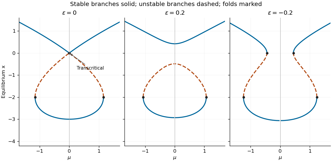
Scalar equilibrium diagrams before and after positive and negative unfolding, with stable branches solid and unstable branches dashed
. Details. 
Write . The entire unfolded diagram is obtained from , with the same dynamical stability sign as before. A saddle-node bifurcation at requires , while a saddle-node bifurcation at requires .
For , the crossing separates into a positive stable branch and a negative unstable branch, with no saddle-node bifurcation near . Three equilibria exist for , and the two negative branches annihilate at the outer saddle-node bifurcations . Outside that interval only the positive stable equilibrium remains. If , the diagram has just that one branch everywhere; equality is the limiting saddle-node bifurcation contact at .
For , let . Two inner saddle-node bifurcations occur at , and two outer saddle-node bifurcations at . For there is a single stable equilibrium below ; for there are three equilibria with stable–unstable–stable ordering; outside the outer saddle-node bifurcations only the positive stable equilibrium remains. The preceding figure shows representative small unfoldings. In particular this unrestricted perturbation destroys the exact transcritical bifurcation crossing.
Put . The planar vector field and its equilibrium eigenvalue data areFor a nonzero equilibrium, use to rewrite the determinant as . These formulas determine the local bifurcations of the imperfect soft Duffing-van der Pol oscillator directly.
When , the origin is a saddle equilibrium for and has determinant for ; the two equilibria are saddle equilibria. They meet the origin in a symmetry-protected pitchfork bifurcation at for . At the origin undergoes a supercritical Hopf bifurcation. To determine criticality, take : averaging gives , so the stable small limit cycle has .
The potential energy of the conservative part and the exact energy balance areAt zero imperfection the stable limit cycle grows to a heteroclinic cycle connecting the two outer saddle equilibria. Near the double-zero point its leading connection curve can be calculated, rather than inferred just from symmetry. In the Hamiltonian system limit the heteroclinic orbit is , andThe weak-damping persistence condition is therefore , not an exact formula at order-one parameters.
Now take ; negative imperfection reflects the phase portrait. The pitchfork bifurcation unfolds into a transcritical bifurcation crossing at and a saddle-node bifurcation at . The latter occurs at . Between those values the origin and are saddle equilibria, while lies in and is a sink or source according to the trace. At , exchanges its saddle equilibrium/non-saddle character with the origin. The double-zero points are now at and .
The original Hopf bifurcation line remains, still supercritical. A second Hopf bifurcation curve occurs on the intermediate nonzero equilibrium:It is important not to assign the same criticality to its entire length. Write , so . Around that center the restoring quadratic coefficient is , the damping linear coefficient is , and . The Hopf criticality for an asymmetric Lienard center calculation gives cubic amplitude coefficientHence it is supercritical for and subcritical for , with a generalized Hopf bifurcation point at . Higher-order terms are needed exactly there. For small imperfection the leading quintic coefficient is positive: writing and using the coordinate that normalizes the potential energy, , with and , the coefficient of in at vanishing cubic coefficient is . Weak-damping averaging therefore supplies the nearby saddle-node bifurcation of stable and unstable limit cycles in the generalized Hopf bifurcation unfolding. None of these small features intersects either requested parameter line.
Globally, the two saddle equilibrium barriers are no longer equal. Their leading energy difference is . The two one-way connections consequently separate; matching their energy differences with the connection integral givesThese weak-damping heteroclinic splitting of a tilted quartic oscillator formulas apply for small with . Between the separated connection curves, the central stable limit cycle terminates in a homoclinic orbit to the lower-barrier saddle equilibrium, for positive imperfection. The simultaneous symmetric heteroclinic-cycle destruction is therefore replaced by two basin-changing one-way connections and a distinct homoclinic orbit loss of the limit cycle. Its period diverges at that loss.
Along , decrease from above one. The sequence is supercritical Hopf bifurcation at ; first heteroclinic orbit; homoclinic orbit loss of the stable limit cycle; second heteroclinic orbit; transcritical bifurcation crossing at zero; saddle-node bifurcation at . The connection locations are global, not obtained by treating the Melnikov approximation as exact. For illustration, direct stable/unstable manifold matching at places them at approximately , respectively. The diagram below gives the qualitative ordering without prescribing those example values for arbitrary imperfection.
Along , the sequence is simply transcritical bifurcation crossing at zero, followed by saddle-node bifurcation at . Before the latter, in the relevant region, so decreases strictly on nonstationary trajectories and there is no periodic orbit or saddle equilibrium loop. After it only a saddle equilibrium remains, which cannot be enclosed by a periodic orbit by the Poincare-index obstruction to a periodic orbit. The origin does not undergo a Hopf bifurcation at , since its determinant there is negative.
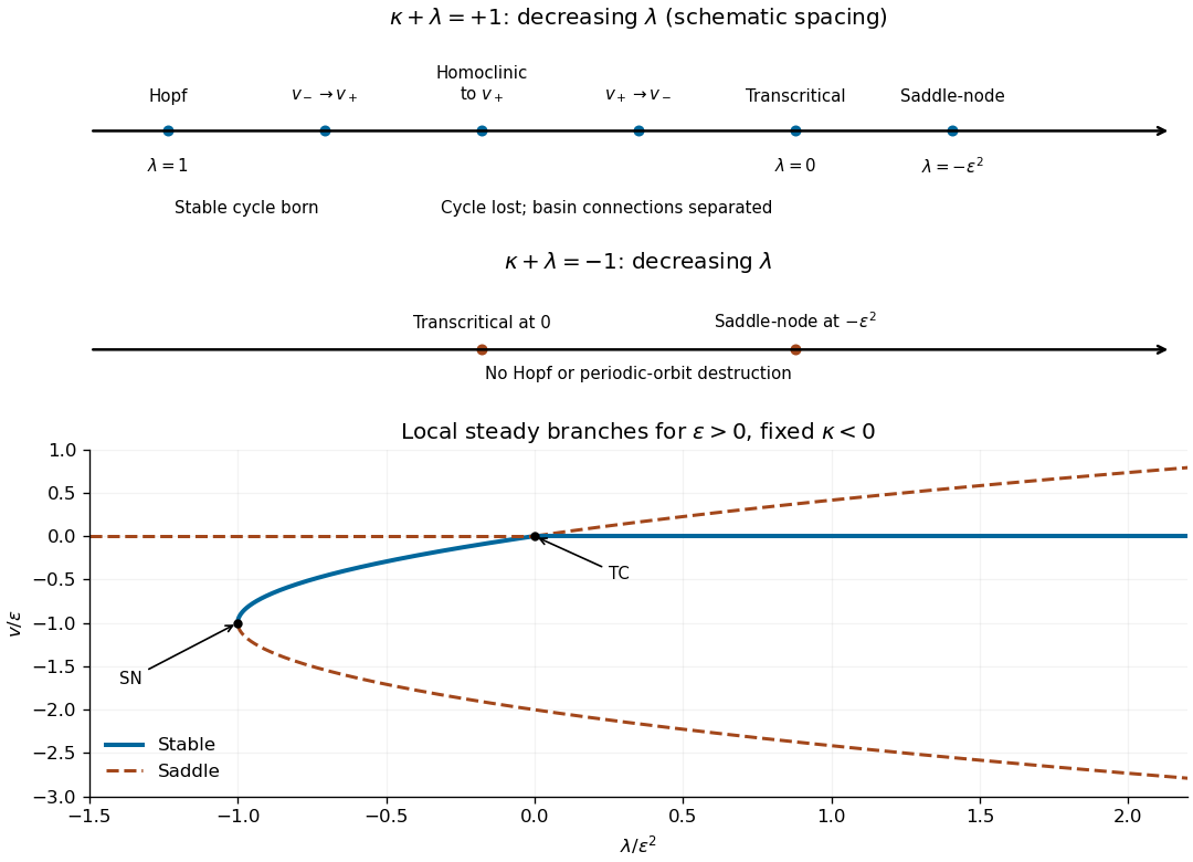
Bifurcation sequences along the two diagonal parameter lines after a small positive reflection-symmetry imperfection; arrows indicate decreasing lambda
. Details. 
Write and use modes satisfying all boundary conditions,The quadratic temperature distortion is retained for the saturation calculation; it does not enter the linear onset. Substitution of the primary modes givesThe determinant vanishes whenThe trace is . Thus no conjugate eigenvalues can cross the imaginary axis away from zero, and the initial instability is stationary, not oscillatory. Indeed for the discriminant is . This is quasistatic vertical-field magnetoconvection: there is no independent magnetic evolution mode that could produce a magnetic-thermal Hopf bifurcation instability.
For a fixed box the other allowed horizontal wavenumbers are , and the actual first threshold is the minimum of their corresponding values. Vertical index replaces by and strictly increases the threshold at fixed horizontal wavenumber, so is selected. The displayed formula describes the prescribed fundamental roll; part (b) optimizes its width.
Put and . ThenThe minimizing condition isIts left side increases strictly for and the neutral curve diverges at both ends, so there is a unique global minimum. For large , and the leading balance is . ThereforeThis is the strong-field wavenumber selection in magnetoconvection scaling. In a box of fixed width one compares the two admissible horizontal wavenumbers bracketing the continuum optimum.
The primary vorticity Jacobian determinant vanishes because . The quadratic temperature Jacobian determinant isThe mean temperature correction therefore obeys . Its Jacobian determinant with the primary streamfunction isProjecting on the retained primary modes gives, with ,For a nonzero steady roll, and . Substitution in the second equation gives, within this truncation,The positive denominator ensures branches only on the supercritical side for every . To verify dynamical stability as well as existence, the critical right eigenvector is ; normalizing the left eigenvector gives linear eigenvalue derivativeQuadratic slaving gives , and projection of its feedback gives the cubic amplitude equationIts nonzero branches are stable in the center direction, while all other eigenvalues remain negative at a simple onset. Reflection about the mid-width sends , so the bifurcation is a supercritical pitchfork bifurcation for all , in the generic case of a single critical roll mode.
The cubic saturation of quasistatic magnetoconvection result is identical in Fourier truncation and perturbation theory at the orders needed here. At quadratic order the only forced mode is precisely the retained horizontally uniform temperature mode. At cubic order its feedback projects on the primary mode with the same coefficient. The generated third vertical harmonic is orthogonal to that primary projection and contributes only to higher-order corrections. Thus both methods give the same linear threshold and cubic solvability condition; the truncated finite-amplitude branch is not an exact solution of the full PDE at all amplitudes.
After one iteration , so work on that invariant sign sheet. For ,since and . This is the signed gluing-map reduction. If an arbitrary initial value of is admitted, the formula applies after that first iterate, not before it. The point represents a separatrix at which the original flow return is singular, even though the scalar map can be extended continuously there.
Let a scalar fixed point have magnitude . If , then and have the same sign; the two lifts are the fixed points and . If , their signs are opposite, and the lift is the period-two orbit . The scalar fixed-point multiplier isThe two-return fixed-point multiplier of the period-two lift is , so in either case dynamical stability requires . The negative fixed point represents one of two mirror-related single-lobe periodic orbits in the flow, whereas the positive fixed point represents a double-lobe periodic orbit.
For , the nearby fixed point is and its fixed-point multiplier tends to zero. Thus two stable single-lobe limit cycles for glue into one stable double-lobe limit cycle for . Their periods diverge as the separatrix is approached; is not a finite-period limit cycle.
For , the small branch instead satisfies and its fixed-point multiplier tends to infinity. Hence one unstable double-lobe limit cycle on splits into two unstable single-lobe limit cycles on . Additional finite-size stable branches depend on the surrounding map; near the resonance with they are resolved by the saddle-node bifurcations in part (c).
For a fixed point write . A saddle-node bifurcation requires both and . For these conditions giveThe second derivative is nonzero at either nonzero saddle-node bifurcation, making it an ordinary saddle-node bifurcation. For , defineThe saddle-node bifurcations occur at and , and three scalar fixed points coexist for . The two outer branches have fixed-point multiplier below one and are stable, while the middle branch is unstable. Negative points lift to two symmetry-related limit cycles, so these scalar branch counts need not equal the number of flow limit cycles. The cusp records coexistence of distinct return-map branches; even outside it a negative branch represents a symmetry-related pair of flow cycles.
If , , thenThis exponentially narrow region ends in a gluing-map cusp at . At its boundaries the graph of is tangent to the diagonal at or , as shown below. At exactly , and gives one stable fixed point for nonzero .
For , the formal saddle-node bifurcation radius is , and the corresponding saddle-node bifurcation parameters also diverge. Thus the near-origin gluing-map cusp lies on the side; the formal large saddle-node bifurcations of the power-law formula on the other side are outside the local gluing-map approximation. They must not be drawn as a second small gluing-map cusp near the origin.
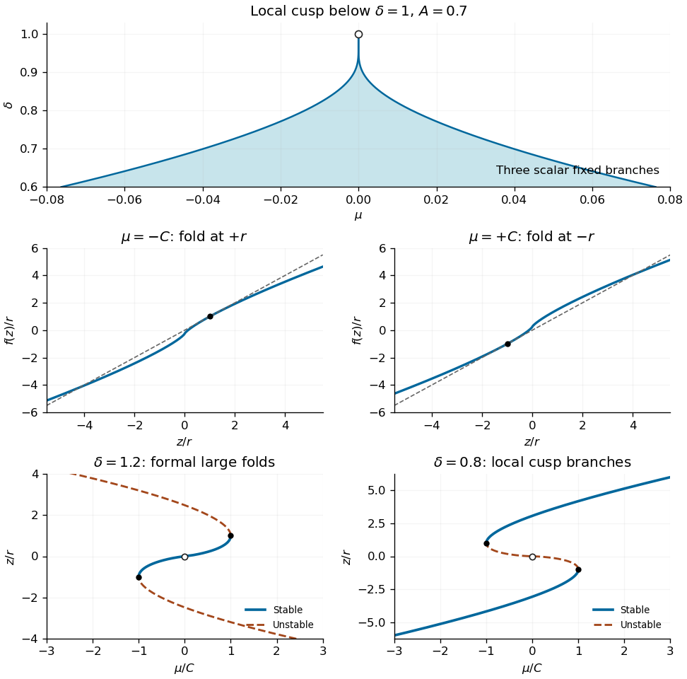
Exponentially narrow gluing-map cusp, tangencies at its two fold boundaries, and stable and unstable fixed-point diagrams on either side of delta one
. Details. 
For , the graph of has a positive maximum at and a negative minimum at . The central branch is stable, while the formal outer branches are unstable. Near the gluing point only the stable central branch is relevant: it crosses from negative to positive , representing the stable two-to-one gluing described in part (b). The formal full power-law diagram has three fixed points between its two large saddle-node bifurcations.
For , the positive branch has its minimum at , while the negative branch has its maximum at . The inner pieces are unstable and outer pieces stable. In the gluing-map cusp interval there is a stable negative branch, a stable positive branch, and an unstable central branch; the unstable branch passes through the singular gluing point with opposite sign to . Outside the gluing-map cusp just one stable outer branch remains. The lower panels of the figure plot these diagrams in fold-scaled variables; dashed lines denote instability and solid lines dynamical stability. Neither diagram has a flip bifurcation, since the scalar derivative is positive wherever defined.
Articles by others on the same topic
There are currently no matching articles.