Multivariate analysis of variance extends analysis of variance to vector responses. For example, a treatment may affect several correlated physiological measurements jointly. Separate univariate tests do not use the correlation geometry and require adjustment if they are interpreted as one multiple-testing procedure. A joint test asks whether group mean vectors differ in any direction.
In a one-way model, take independent , , , with a common positive-definite covariance. Put , and let and be group and overall sample means. The within-group and between-group scatter matrices areExpanding around each group mean makes the cross terms vanish, giving total scatter . To test , use the Wilks lambda statisticwhere solve the generalized eigenvalue problem and is nonsingular. Under the alternative, maximize the normal likelihood at the group means and covariance ; under the null, use the overall mean and covariance . Their likelihood ratio is , so small rejects equal means. Under the null, orthogonal projections of the Gaussian data give independent and , supplying its null calibration. Here is nonsingular almost surely when . Merely having more total observations than responses is not enough if group fitting consumes too many statistical degrees of freedom.
The test is invariant under a nonsingular linear change of response coordinates: both determinants acquire the same factor . The directions associated with large identify mean separation relative to residual variability. With one response it becomes the ordinary ANOVA F-test. With two groups, writing and , the version using Hotelling's T-squared statistic iswith . This formula demonstrates explicitly how the covariance weights a group difference.
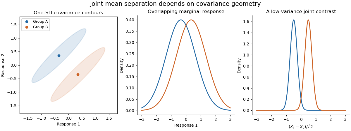
The sketch shows hypothetical groups with strongly positively correlated responses and mean separation along their low-variance contrast. Marginal comparisons can look weak even when the joint comparison is informative. The ellipses represent individual-response covariance, not confidence regions for the means. Independence of observations, approximate multivariate normality and common covariance are substantive assumptions; outliers and unequal covariance can invalidate the usual calibration. Follow-up contrasts can identify the affected responses or groups, with appropriate multiplicity control. MANOVA uses shared covariance to test a multivariate mean difference, rather than testing unrelated coordinates in isolation.
Factor analysis models a large set of correlated measurements using a smaller collection of shared latent factors and variable-specific variation. A classical orthogonal factor model isTake , centered errors, and positive specific variances for the inverse-covariance and likelihood formulas below. The factor loadings form the matrix , and the model covariance isThus for , ; the common latent factors explain off-diagonal correlation. The communality of variable is , and . For standardized variables this is . The specific variance represents measurement noise or genuinely unshared variation; it is not another common latent factor.
This differs from principal component analysis. A principal component maximizes projected total variance and is a determined linear score after choosing its direction; a factor model attempts to explain shared covariance while reserving diagonal specific variance. Low-dimensional PCA truncation can help initialize a factor fit, but it does not justify setting all specific variances to zero. Latent factors are unobserved, not directly observed scores. When the latent factors and the errors are jointly Gaussian, their conditional mean iswhich supplies one factor-score estimate, with remaining uncertainty. This follows from the block conditional normal formula in Question 1; it does not make the latent factor uniquely recoverable from one observation.
For the Gaussian likelihood, use the empirical covariance . Fit the factor model by minimizing subject to admissible specific variances. Other approaches estimate communalities and extract latent factors from the reduced correlation matrix. Choose using substantive plausibility, a scree plot, fitted residual correlations and model-fit assessment. Under local identifiability, a likelihood goodness-of-fit count for the covariance model iswhere the subtracted rotational dimension must be removed from the loading parameter count. This count alone does not establish identifiability, and boundary fits with zero specific variance need special care.
Factor rotation addresses interpretability and nonuniqueness. For every orthogonal matrix , replace by ; then , so the fit is unchanged. The absolute orientation of unrestrained latent factors is therefore not identified by the covariance. Varimax rotation chooses orthogonal axes favoring a simple pattern of large and small squared loadings. Oblique rotation can permit correlated latent factors, provided their covariance is transformed consistently. Sign changes and permutations are further harmless relabelings; an interpretation must state its chosen convention.
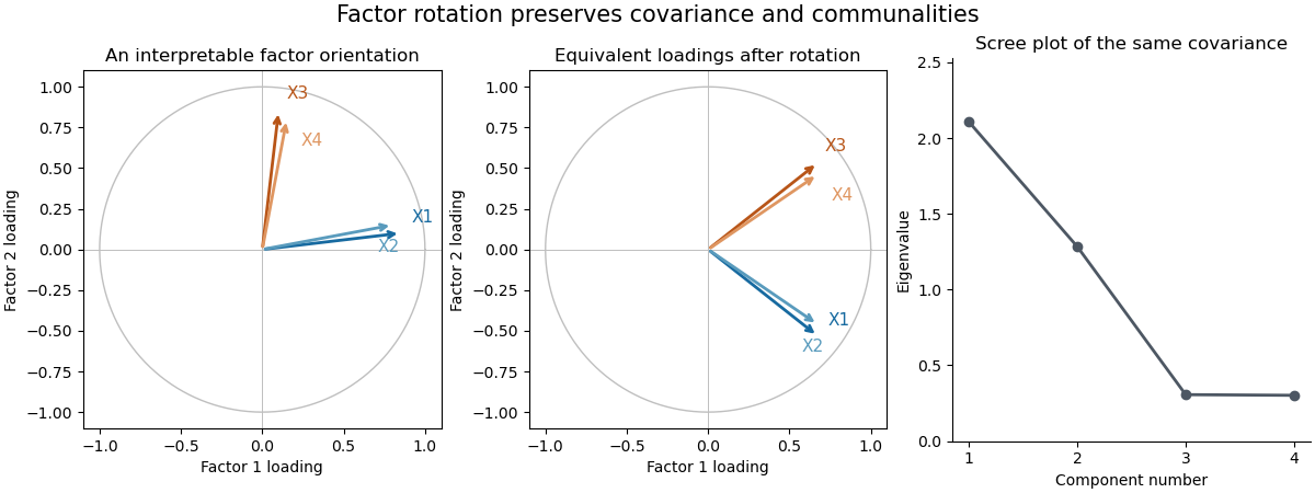


The sketch uses four standardized hypothetical measurements sharing two orthogonal latent factors. Rotating the factor coordinates changes the loading descriptions while preserving every implied covariance and communality; the scree plot belongs to that same constructed covariance matrix. Factor analysis separates shared variation from specific variance, and its latent factors require an identifying or interpretive orientation.
Cluster analysis groups observations without given class labels. It starts by deciding what similarity means, usually through a dissimilarity matrix. Euclidean distance is natural for comparable continuous coordinates; a Mahalanobis distance can account for differing scales and correlations when a meaningful nonsingular covariance estimate is available. Scaling and variable selection can change the groups. Binary, ordinal or categorical data may need a different dissimilarity, rather than arbitrary numerical codes and Euclidean distance.
Agglomerative hierarchical clustering begins with singleton groups, repeatedly merges the pair with smallest intergroup dissimilarity, and records the merges in a dendrogram. The height represents the algorithm's merge criterion. Cutting the dendrogram gives partitions at different resolutions, and merges cannot subsequently be reversed. In single-linkage clustering, the criterion is the nearest cross-pair distance; this detects chains and nonconvex groups, but a thin bridge can connect otherwise separated clouds. Complete-linkage clustering uses the farthest cross-pair distance and tends to produce compact groups, at the cost of sensitivity to extreme points. Average-linkage clustering uses the mean cross-pair distance, lying between these two criteria for a given pair of clusters.
For squared Euclidean geometry, Ward clustering merges the pair that least increases the within-group sum of squares. Expanding deviations about the merged mean givesThis favors low within-group dispersion, but interpreting it as a sum-of-squares increase requires Euclidean data. Different software may plot a rescaled height, so the vertical units of a dendrogram from Ward clustering must be stated.
A nonhierarchical alternative is k-means clustering. For a prescribed , minimizeAt fixed assignments, expanding squared distances or differentiating shows that the minimizing is the group mean. At fixed centroids, each point is assigned to a nearest centroid. Alternating these operations does not increase ; with a consistent tie rule and nonempty groups it reaches a locally stable partition. Initialization matters, so use multiple starts, and give an explicit rule for empty groups. It favors roughly spherical clusters and is sensitive to outliers and scaling. It cannot be expected to reproduce a nonconvex single-linkage partition.
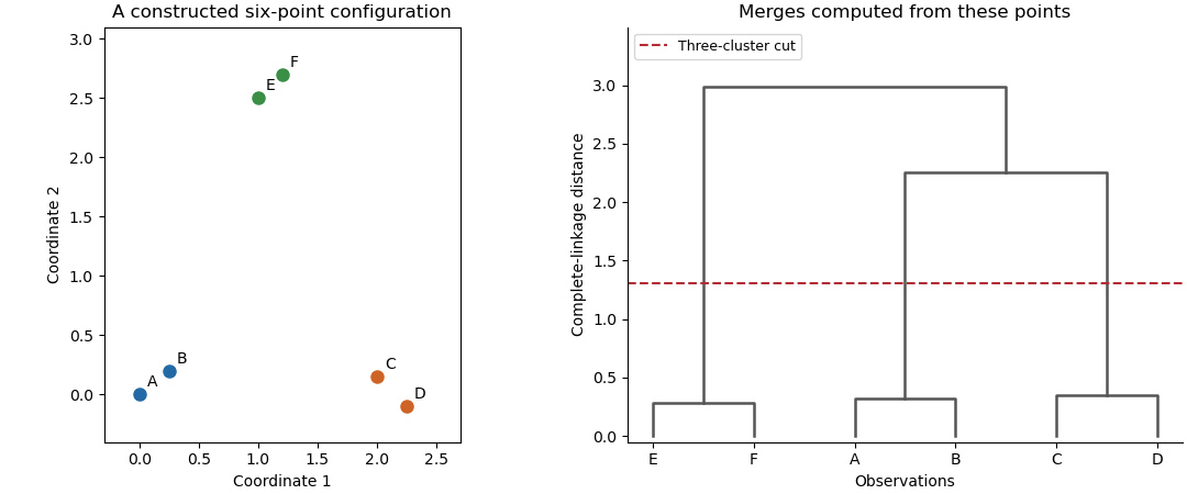
An original point configuration and its computed complete-linkage dendrogram with a three-cluster cut
. Details. 
The sketch displays a constructed point configuration and the complete-linkage merges computed from its actual Euclidean distances. A cut between the within-pair and between-pair merge heights yields three groups. Such visual separation is useful evidence, not proof of a uniquely correct number of populations. Select a resolution using subject knowledge, stability under resampling, separation diagnostics or the change of with . Clustering always gives a partition even for unstructured data, and different distance or linkage choices can yield different sensible summaries. Clustering is an exploratory construction whose conclusions depend on the geometry and the chosen resolution.
Articles by others on the same topic
There are currently no matching articles.