Past exam of the mathematics course of the University of Cambridge / 2007 / iii / Paper 51 (Advanced Quantum Field Theory)

For one Grassmann variable, define the Berezin integral by $\int d\theta 1=0$ and $\int d\theta \theta =1$, extending linearly. Since ${\theta }^2=0$, these rules determine it on every polynomial. With several Grassmann variables, integrate from the rightmost differential first. Equivalently, $\int d{\theta }_n\cdots d{\theta }_1$ extracts the coefficient of ${\theta }_1\cdots {\theta }_n$ in that order. Repeated indices give zero, while permuting distinct generators gives the fermionic sign of that permutation. Hencewhere $\epsilon$ is the Levi-Civita symbol.

For the doubled variables, fix the paired measure orientation byThe exponential in the Grassmann Gaussian integral has a finite Taylor expansion. Only its term of degree $2n$ survives integration. Each barred and unbarred index must occur exactly once; the $n!$ orders of the even bilinears cancel the Taylor factorial. Reordering the unbarred indices gives the determinant permutation sign. ThereforeThis identity holds even for a singular matrix. The normalized expectations below require $B$ invertible.

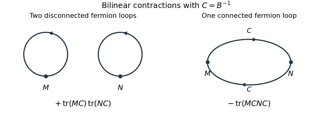
Put $C=B^{-1}$. Differentiating with respect to $B_{ji}$ inserts $-{\bar{\theta }}_j{\theta }_i={\theta }_i{\bar{\theta }}_j$. The derivative of a determinant then gives the ordered Grassmann Gaussian contractionsDifferentiate once more, using $\partial C_{ij}/\partial B_{lk}=-C_{il}{C}_{kj}$. The result isThe minus sign is the interchange sign in the fermionic Wick theorem. In particular $⟨\bar{\theta }M\theta ⟩=-\mathrm{tr}(MC)$. Reordering each barred-unbarred pair in the product and contracting the indices givesThe covariance of Grassmann bilinears is the connected second term. Its Feynman diagram is one oriented fermion loop through both insertions; the first term has two separate fermion loops, one at each insertion. Each closed fermion loop contributes a minus sign, so two loops give a plus and one gives a minus.

For the Dirac field, write $D=\gamma \cdot \partial +m$ and use signature $(-,+,\dots ,+)$, consistent with the denominator in the question. A finite regulator turns the free fermionic path integral into the same Gaussian problem with $B=iD$, because $e^{iS}=e^{-i\bar{\psi }D\psi }$. The time-ordered product covariance is consequently $(i{D}_F{)}^{-1}=-i{D}_F^{-1}$, where the subscript specifies the Feynman i-epsilon prescription.

With the Fourier transform convention $\psi (x)=\int d^{d}p(2\pi {)}^{-d}{e}^{ip\cdot x}\tilde{\psi }(p)$, the derivative kernel is $i\gamma \cdot p+m$. The gamma matrices obeysince their anticommutator makes $(\gamma \cdot p{)}^2=p^{2}I$. Thus the mostly-plus Dirac propagator with a real derivative kernel isFor $p^2=-p_0^2+{\mathbf{p}}^2$, the denominator is $p_0^2-{\mathbf{p}}^2-m^2+i0$. Its positive-energy pole is below and negative-energy pole above the real axis, giving time ordering. Here $S_F$ is defined without the leading factor $i$, as in the question; conventions that include that factor in the name Dirac propagator give the same covariance.

For $m^2>0$ and initially $\Re n>d/2$, Schwinger parameterization and the supplied Gaussian integral giveSubstitute $u=\alpha m^2$ to obtain the Euclidean massive loop integralFor a positive integer $n$, $\Gamma (n)=(n-1)!$. Outside the convergence region this expression defines its meromorphic continuation, used in dimensional regularization.

Combine the two denominators with a Feynman parameter and shift $k$ by $(1-x)p$. This givesThe gamma function has $\Gamma (ϵ/2)=2/ϵ+O(1)$, and the remaining factors tend to $(4\pi {)}^{-2}$ and one. Hence the massive scalar bubble pole in four dimensions isThe pole is independent of the external momentum, as required for a local quartic counterterm.

Use the mostly-plus Minkowski metric and expand $e^{iS}$. The momentum-space Feynman rules are: an internal scalar propagator $i/(-p^2-m^2+i0)$; a four-scalar interaction vertex $-i{\mu }^{ϵ}\lambda$; a momentum conservation delta function at each vertex; and $\int d^{d}k/(2\pi {)}^d$ per independent loop momentum. Divide by the Feynman-diagram symmetry factor. All momenta can be taken incoming. External propagators are omitted when computing an amputated one-particle-irreducible vertex.

The connected one-loop one-particle-irreducible Feynman diagrams are the two-point tadpole diagram and the three four-point bubble diagrams, in the $s,t,u$ channels. Each has symmetry factor $1/2$. A tadpole attached to an external leg through a single bridge would be reducible, so is excluded here.

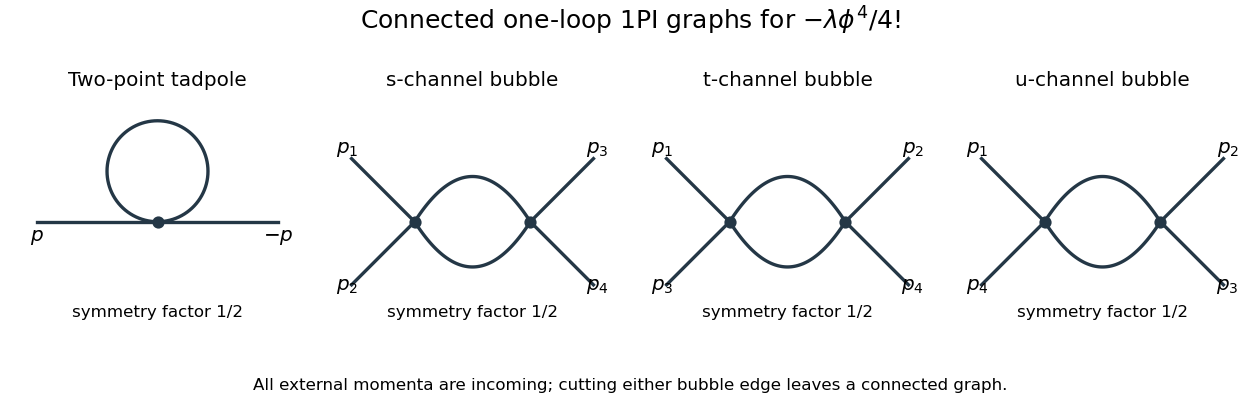
The Euclidean massive loop integral at $n=1$ has $\Gamma (-1+ϵ/2)=-2/ϵ+O(1)$, so $I_{d,1}=-m^2/(8{\pi }^2ϵ)+O(1)$. Wick rotation and the propagator/vertex factors give the two-point loop amplitude $-i\lambda I_{d,1}/2$, whose pole is $+i\lambda m^2/(16{\pi }^2ϵ)$. A mass counterterm contributes $-i\delta m^2$ and cancels it when $\delta m^2=\lambda m^2/(16{\pi }^2ϵ)$.

Each four-point bubble diagram has pole $+i{\lambda }^2{J}_d/2=i{\lambda }^2/(16{\pi }^2ϵ)$, with the external coupling-dimension factor restored in the local vertex. Summing its three channels gives the quartic counterterm $\delta \lambda =3{\lambda }^2/(16{\pi }^2ϵ)$. Therefore the one-loop massive phi-fourth counterterms are exactlyThere is no one-loop wave-function renormalization, since the tadpole is independent of external momentum. Vacuum graphs would additionally require a vacuum-energy subtraction.

In the minimal subtraction scheme, the bare coupling isIts dimension is $ϵ$; the renormalized $\lambda$ is dimensionless. Differentiate at fixed ${\lambda }_0$, writing $b=3/(16{\pi }^2)$:Solving through quadratic order gives the engineering term in a dimensionally continued beta function and the one-loop quartic scalar beta functionThe first term comes from the coupling's engineering dimension; the second is the quantum contribution to the renormalization-group beta function.

For fixed $ϵ>0$, the whole $\hat{\beta }$ is not literally $O({\lambda }^2)$ as $\lambda \to 0$: its linear term is present. Interpret the final instruction as keeping terms through quadratic order. Set ${\lambda }_{\ast }=ϵ/b=16{\pi }^2ϵ/3$. Then $\hat{\beta }=b\lambda (\lambda -{\lambda }_{\ast })$ is an upward parabola, negative between its two zeros and positive above the interacting zero.

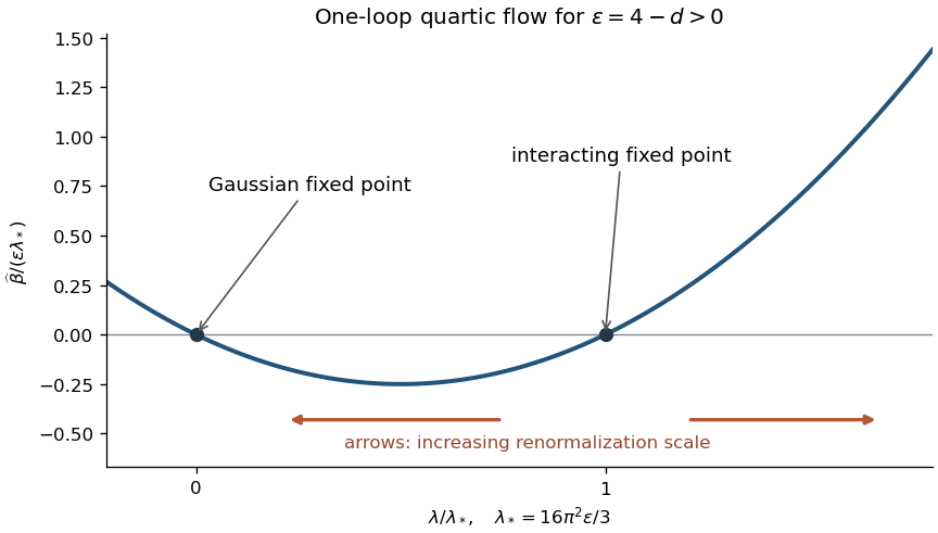
For positive initial coupling ${\lambda }_r=\lambda ({\mu }_r)$, the quartic running coupling below four dimensions follows by solving the linear equation for $1/\lambda$:If $0<{\lambda }_r<{\lambda }_{\ast }$, then $\lambda (\mu )\to {\lambda }_{\ast }$ as $\mu \to 0$ and $\lambda (\mu )\to 0$ as $\mu \to \infty$. If ${\lambda }_r={\lambda }_{\ast }$ it stays fixed; the zero solution also stays fixed. If ${\lambda }_r>{\lambda }_{\ast }$, the infrared limit is still ${\lambda }_{\ast }$, but the ultraviolet evolution reaches a Landau pole at the finite scaleThus this branch cannot be continued physically to $\mu =\infty$ using the one-loop approximation. These are statements about the quartic coupling direction. The Wilson-Fisher fixed point of the full scalar theory also has a thermal relevant direction at the Wilson-Fisher fixed point; approaching the critical theory requires mass tuning. For negative initial coupling, the quartic potential is unstable: the same formula tends to zero from below in the ultraviolet and reaches a pole at finite scale toward the infrared.

With $Z[J]=e^{iW[J]}$, the logarithm $W$ is the connected generating functional. Its derivative $\phi =\delta W/\delta J$ is the mean field. The specified Legendre transform satisfies $\delta \Gamma /\delta \phi =J$, and the quantum effective action generates amputated one-particle-irreducible vertices by further functional derivatives. In this question $\Gamma =-W+\int J\phi$ is the negative of the commonly used Minkowski effective-action convention; consequently its tree term is $-S[\phi ]$. Its diagrammatic content is unchanged if the convention is used consistently.

Expand the action around a stationary background in the presence of the source. For $\varphi =\phi +f$, integration by parts givesThe linear term vanishes at the tree-level saddle, $\delta S/\delta \phi +J=0$. Keeping the Gaussian fluctuation approximation, and fixing the field-independent normalization, givesto one-loop order. The shift from the tree saddle to the exact mean field cancels from the tree Legendre transform at this order. Hence the one-loop scalar effective action in the question's convention isThe functional determinant has a Feynman i-epsilon prescription before Wick rotation. Higher loops come from the omitted cubic and higher fluctuation vertices.

To see the one-loop one-particle-irreducible Feynman diagrams, write $\Delta ={\Delta }_0+U(\phi )$. Its determinant expansion isEach trace closes a single scalar loop, with propagators ${\Delta }_0^{-1}$ and background insertions $U$. No internal edge is a bridge, so these graphs are one-particle irreducible. Expanding the background factors produces their external legs.

For a constant $\phi$, set $A=V^{\prime \prime }(\phi )>0$. The quantum effective potential is defined here by $\Gamma [\phi ]=\int d^{d}x{V}_{\mathrm{eff}}(\phi )$. A plane-wave basis diagonalizes $\Delta$, and the supplied Wick rotation converts its correction per unit volume toHere the power of the renormalization scale keeps the continued integral in four-dimensional units. The Gamma function recurrence and expansion giveConsequentlyThe divergence is local, so subtract it with a potential counterterm. In the modified minimal subtraction scheme, remove its associated $\gamma -\log 4\pi$ constants as well. The one-loop scalar effective potential becomesup to an arbitrary field-independent vacuum-energy constant. Another allowed finite subtraction replaces the nonlogarithmic constant. Restoring a loop-counting parameter would multiply the displayed correction by $\hslash$. The logarithm assumes positive curvature $A$; a background with negative curvature requires an analytic continuation and can have an imaginary part signalling instability.

The quartic case is special because of quartic closure of scalar effective-potential counterterms. If $V$ has degree at most four, then $V^{\prime \prime }$ has degree at most two and $(V^{\prime \prime }{)}^2$ has degree at most four: its pole is removable by the original polynomial couplings and a constant. For example, $V=m^2{\phi }^2/2+\lambda {\phi }^4/4!$ givesThe last two terms reproduce the one-loop massive phi-fourth counterterms, and the first is a vacuum-energy subtraction. A degree-$r$ potential with $r>4$ instead generates degree $2r-4>r$, forcing new operators. This is the potential-level manifestation of power counting in quantum field theory and four-dimensional renormalizability, even though the finite effective potential itself need not remain polynomial.

Let $R_i(x)={\partial x_{g(\theta )}/\partial {\theta }_i|}_{\theta =0}$ be the infinitesimal orbit tangent vectors. Since $F_j(x_0)=0$, Taylor expansion givesThis explains the stated linearization. For a linear group representation, $R_i(x)=t_{i}x$ in the corresponding action convention.

Two assumptions are implicit in the advertised integration formula. The slice must be regular, and the determinant sign must be fixed if the absolute value is omitted. Uniqueness alone does not imply regularity: translations on the line with $F(x)=x^3$ have a unique gauge-fixed representative but $M(0)=0$. For ordinary real integration the Dirac delta distribution change-of-variables formula uses $|\det M|$. The choice $F(x)=-x$ instead has a unique regular zero and negative determinant, illustrating why its sign cannot simply be dropped.

Assume a regular gauge slice with one representative on each orbit, and choose the action convention $(x_{g_0}{)}_{g(\theta )}=x_{g(\theta )g_0}$, matching the specified right-invariance of Haar measure. For the unique $x_0=x_{g_0}$ with $F(x_0)=0$, put $g=g(\theta )g_0$. The Haar density is one at the identity, so changing from $\theta$ to $F$ near the unique zero givesThe integral is orbit invariant by the right-invariance of Haar measure. Thus $\Delta (x)=I(x{)}^{-1}$ is also orbit invariant, and on the gauge slice it equals $|\det M(x)|$. Insert $1=\Delta (x)I(x)$ into the original integral and use its invariant volume measure and invariant $f$:In the second line set $y=x_g$. This proves the finite-dimensional Faddeev-Popov gauge reductionChoose a positive orientation of the regular slice to obtain the question's $\det M$ form. If the group volume is infinite, its cancellation in normalized quantities is formal or regulated. Multiple intersections and residual zero modes invalidate the simple identity; in a gauge theory these are the Gribov ambiguity and residual gauge transformations.

The Yang-Mills action counts every gauge orbit redundantly in its path integral, and its quadratic gauge-field operator has gauge zero modes. A gauge fixing condition removes this redundancy, while the Faddeev-Popov determinant supplies the orbit-to-slice Jacobian. This is a local perturbative construction with the same regularity qualifications as the finite-dimensional derivation.

Take the linear condition $G[A]=F^{\mu }{A}_{\mu }$. Under an infinitesimal gauge transformation $\delta A_{\mu }=D_{\mu }\omega$, its change is $\delta G=F^{\mu }{D}_{\mu }\omega$. Hence the Faddeev-Popov operator is $\mathcal{M}[A]=F^{\mu }{D}_{\mu }$. For Lorenz gauge, $F^{\mu }={\partial }^{\mu }$. The gauge covariant derivative acts in the Adjoint representation.

Average the sharp constraint $G=h$ over $h$ with Gaussian weight $\exp [-i\int h^2/(2\xi )]$. This replaces it by $\exp [-i\int G[A{]}^2/(2\xi )]$. The Gaussian gauge fixing with an auxiliary field identity rewrites that factor asby completing the square. The bosonic Nakanishi-Lautrup field $b$ is nondynamical: its algebraic field equation is $b=-G[A]/\xi$. At $\xi =0$ it is a Lagrange multiplier enforcing $G[A]=0$.

The Grassmann Gaussian integral exponentiates the determinant, up to a field-independent phase, asThe independent anticommuting Faddeev-Popov ghost field $c$ and Faddeev-Popov antighost field $\bar{c}$ are spacetime scalars in the Adjoint representation. They represent the Jacobian and do not describe physical external fermions. Combining these factors givesThe parameter $\xi$ selects the Gaussian averaging of the gauge condition. In an anomaly-free regulated treatment, physical gauge-invariant observables are independent of this choice. One way to express this is BRST symmetry: with $sA=Dc$, $s\bar{c}=-b$ and $sb=0$, the gauge and ghost terms are $s[-\bar{c}\cdot (G+\xi b/2)]$. The ghost transformation supplies the off-shell nilpotence of the Yang-Mills BRST quartet, and gauge-fixing parameter independence from BRST symmetry explains why these auxiliary fields do not change the physical content.