The dual linear program is the minimization problemIndeed, for the optimization Lagrangian bounds the primal objective above on its feasible points. Its supremum over is finite precisely when , and then equals . The two labelled parts below establish the relevant weak duality and strong duality conclusions.
For the subsequent infeasibility argument, introduce nonnegative slack variables and the convex coneThis is generated by the columns of and the coordinate vectors. Here is why this finitely generated cone is closed. Any representation with a minimal number of positive coefficients uses linearly independent generators: otherwise subtract a suitable multiple of a dependence until one positive coefficient vanishes, preserving nonnegativity. For each fixed independent selection of generators, its nonnegative combinations form a closed set, because the inverse coordinate map on its span is continuous. There are finitely many selections, so their union is closed. This is the closedness of finitely generated cones used in Farkas' lemma.
When the primal linear program is infeasible, . Let be the nearest point of to , and set . The minimizing property gives for every . Taking gives . ConsequentlyIn particular and . Rescaling by the positive number produces the requested Farkas' lemma certificate:Now a feasible point of the relaxed inequalities would satisfySince , the sum of the nonnegative is positive. Thus robust infeasibility under uniform constraint relaxation givesThe ellipsoid method makes progress by reducing the volume of a containing ellipsoid. A nonempty linear polyhedron may have empty interior, so small volume alone cannot certify that the original system is infeasible. Relaxing the inequalities remedies this difficulty, but must not make an infeasible system appear feasible. The displayed positive gap proves exactly that sufficiently small relaxations preserve infeasibility. For rational input, determinant bounds give a Farkas' lemma certificate of polynomial encoding length, so a sufficiently small rational relaxation can be chosen from the input encoding length. Together with a bounding box and bounds on the volume of a relaxed feasible system, this lets the ellipsoid method distinguish infeasibility from a feasible system of very small or zero original volume in polynomial time. The certificate argument alone does not assert a polynomial precision bound for arbitrary unencoded real coefficients.
Fix a primal feasible point . For every dual feasible point , nonnegativity and the primal and dual inequalities giveHence the dual objective is bounded below by wherever it is feasible, which is weak duality. This is the meaning of “bounded” in this assertion; it does not say that the dual feasible set is bounded, or that it is nonempty. For example, with , , and a single variable, the primal is feasible and unbounded above, while its dual would require and is infeasible.
Let the finite primal supremum be . First it is attained. The setis a finitely generated cone, hence closed by the argument in the root Solution. For a sequence of primal feasible points whose values approach , the pairs belong to . Their limit therefore belongs to . It gives a feasible point with , so necessarily .
Let index the tight primal inequalities at and let index its zero coordinates. Consider the closed convex cone generated by for and for . If were outside this cone, separation from a closed convex cone would give a direction withFor sufficiently small positive , remains a feasible point: the active constraints have the required signs, and every inactive constraint retains its positive slack. Its larger objective contradicts optimality. Therefore there are , supported on , and , supported on , such thatThis makes a dual feasible point. Moreover, the support restrictions giveTogether with weak duality, this proves strong duality and dual attainment:
Encode a vertex of a polytope by three bits: bit records whether the lower or upper bound of coordinate is tight. Every choice is possible because , and the triangular active equations determine that vertex of a polytope uniquely. Its three adjacent vertices of a polytope are obtained by changing one bit. The geometric Bland pivoting rule specified here chooses the smallest-index active facet that can be left while increasing . It produces the following path; the final column records the facet left on arrival at the next vertex of a polytope:For example, at the origin all three outgoing edges improve the objective, but leaving facet 1 has priority. At bit string , switching bit 2 decreases , so the rule switches bit 1, leaving facet 2. At , neither of the earlier-coordinate switches improves , so the rule finally leaves facet 5. The upper face reverses the direction in which changes of improve , and the remaining three horizontal pivots follow. The objective values in the table are strictly increasing for the stated range of .
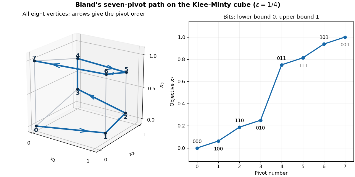
Seven Bland pivots through all eight vertices of the Klee-Minty cube, with epsilon equal to one quarter
. Details. 
Thus the simplex method takes seven pivots although the optimum is directly adjacent to the starting point. The same Klee-Minty cube in dimensions has inequalities and vertices of a polytope. On its lower last-coordinate face, increasing means increasing , and the first coordinates follow the corresponding lower-dimensional path before the last-coordinate facet can be left. On the upper face, increasing means decreasing , and the smallest-index rule traverses that path in reverse. The reverse-path assertion follows by the same induction, interchanging maximization and minimization on each face. Hence the pivot count satisfies , , andThe usual Bland pivoting rule prevents cycling, including degenerate pivots, but this exponential example shows that it does not give a polynomial worst-case pivot bound. For rational fixed , the constraints have polynomial encoding length. Arithmetic cost per pivot does not remove the exponential obstruction.
For a lower bound that applies to every pivot choice, use and maximize , starting at the origin. Each edge of this cube changes only one coordinate, whereas the unique optimal vertex of a polytope is . Every coordinate must therefore be changed along at least one edge. Every route of adjacent pivots takes at least pivots, and every strictly improving route takes exactly .
For Dantzig pivot rule, the rate is the objective increase per unit entering nonbasic variable, as in standard reduced cost pricing. Rescale the three coordinates byThe transformed linear program still maximizes , now with boundsWhen the active facet for coordinate is freed, the other active equations give . The positive rates per unit are thereforefor , respectively. Equivalently, use the nonnegative lower- and upper-bound slack variables of these displayed, normalized inequalities: freeing coordinate changes its entering slack by . Thus Dantzig pivot rule chooses the lowest coordinate index among improving edges and follows the same seven-pivot path. In dimensions set ; the rates give the same pivots. These statements concern coordinate/slack pricing, not objective increase per unit Euclidean edge length, which defines a different pivot rule.
In a minimum-cost flow problem, a directed graph has arc flows , unit costs , lower and upper capacities , and net supplies summing to zero. The linear program minimizes subject to the flow balances and .
Give each graph vertex a network dual potential . With the outgoing-minus-incoming oriented incidence matrix , the optimization Lagrangian isMinimizing over the capacity intervals is separable. A candidate feasible flow minimizes this optimization Lagrangian if it takes its lower bound whenever the network reduced cost is positive, its upper bound whenever that network reduced cost is negative, and any allowed value when that network reduced cost is zero. Equivalently, for arcs with distinct lower and upper bounds,For every other feasible flow , these conditions give . This proves the Lagrangian sufficiency theorem certificate, rather than merely stating the capacitated flow optimality conditions.
Put . The four flow balances determineIntersecting the four capacity intervals gives . In particular,is a feasible flow. Write . Its cost along the feasible interval isHence is optimal precisely when . A network dual potential certificate isThe three interior arcs have zero network reduced costs and , which has the required nonnegative sign at its lower capacity.
For the network simplex algorithm, start with the network simplex tree basis consisting of arcs , and fix nonbasic arc at its lower bound 2. These are exactly the potentials just found. If , no improving pivot is needed. If , arc enters and its fundamental graph cycle increases all four flows by the same amount. At the remaining upper capacities are , so the simplex ratio test allows an increase of 2. Arc reaches its upper bound and leaves the tree. The new network simplex tree basis has arcs , with potentialsNow only the nonbasic arc has a possibly nonzero network reduced cost, namely . It is at its upper bound, so the sign is optimal. Thus for all real costs the complete answer isWhen , both endpoint basic feasible solutions and every intermediate feasible flow have the same cost.
To count basic solutions, a network simplex tree basis omits one arc of the four-cycle and fixes that arc at either bound. The possibilities areThere are eight tree/bound basic representations, seven distinct basic flow vectors, and two basic feasible solutions. The distinction in the first count matters: the upper bounds on and both give the identical flow at . Thus if “basic solutions” counts vectors rather than basis representations, the answer to (i) is seven; the frequently used count of basis/bound choices is eight. The answer to (ii) is unambiguously two, since only satisfy all capacities.
Assume the finite graph is connected, as is necessary for a spanning tree to exist. For a disconnected graph, the same procedures operate separately on its connected components of a graph and produce a minimum spanning forest.
Let be a minimum spanning tree. If it omitted the unique lightest edge across the specified cut of a graph, adding would make exactly one graph cycle: the graph path in between its endpoints, followed by . Since those endpoints are on opposite sides of the cut of a graph, that graph path contains another crossing edge . Distinct weights give . The graph is still a spanning tree, but has smaller total weight, contradicting minimality. Thus every minimum spanning tree contains , the minimum spanning tree cut property.
Prim algorithm starts from one graph vertex, repeatedly choosing the lightest edge from the reached graph vertices to an unreached graph vertex. Connectivity ensures that such an edge exists until all graph vertices have been reached. Each choice adds one new graph vertex and creates no graph cycle. By the minimum spanning tree cut property, every chosen edge belongs to every minimum spanning tree. After choices the selected edges form a spanning tree, necessarily a minimum spanning tree.
For Kruskal algorithm, suppose the next accepted edge joins two different components of the current forest, and let be one of those components. No previously considered lighter edge crosses : an accepted one already joins graph vertices within a current component, while a rejected one had its endpoints connected when it was rejected and therefore still has them in a single current component. Consequently is lightest across the cut of a graph defined by . The minimum spanning tree cut property again places every accepted edge in every minimum spanning tree. At termination the accepted forest must be connected, since otherwise a crossing edge of the original connected graph would have been accepted when considered. It is therefore a minimum spanning tree.
This reasoning also proves the minimum spanning tree is unique. Either procedure produces a spanning tree all of whose edges belong to every minimum spanning tree; another minimum spanning tree cannot have any different edge.
For the minimum spanning tree cycle property, suppose a spanning tree contained the unique heaviest edge of a graph cycle . Removing splits into two components. The remainder of connects the endpoints of , so it contains an edge across these components. This edge cannot belong to , and . Hence is a lighter spanning tree. Thus no minimum spanning tree contains .
Finally consider the reverse-delete algorithm, processing edges from largest to smallest weight. Whenever an edge is retained because its deletion would disconnect the current graph, it is a bridge in a graph; deleting other edges later cannot create an alternative path around it, so it remains a bridge in a graph. If a currently processed edge is deletable, it lies on a current graph cycle. None of that graph cycle's other edges can be an earlier retained heavier edge, since those are bridges in a graph. Thus all other edges on the graph cycle are lighter than . The minimum spanning tree cycle property says that deleting removes no edge of any minimum spanning tree of the original graph. Throughout, connectivity and the presence of the unique minimum spanning tree are preserved. At termination a surviving graph cycle is impossible: any of its edges was deletable when considered, since that entire surviving graph cycle already existed then. The final connected graph is a tree, and hence is exactly the minimum spanning tree.
Use a complete directed graph on cities, with integral arc costs and a threshold . A symmetric cost matrix also represents the undirected travelling salesman problem by orienting a tour. Let the binary variable indicate that city follows city , and forbid self-arcs. The decision integer programming formulation asks whether the following system has a solution:The in-degree and out-degree equations make the selected arcs a cycle cover of a directed graph. Any proper graph cycle on a city set would violate its subset inequality, so the selected arcs form one Hamiltonian cycle. Conversely, a Hamiltonian cycle obeys every inequality: a proper subset cannot contain all the successor arcs of its graph vertices. Thus the binary feasibility system is equivalent to the decision travelling salesman problem. The subset formulation has exponentially many inequalities, which is harmless for this formulation; verifying a proposed tour does not require listing them.
To call this decision problem NP-complete means two separate things. It belongs to NP: a yes-instance has a polynomial-length certificate in computational complexity, namely the cyclic ordering of the cities, and a deterministic algorithm checks distinct visits, the return to the start, and the total cost in polynomial time in the binary input length. It is also NP-hard: every decision problem in NP has a polynomial-time many-one reduction to it, preserving yes and no answers. This is a statement about worst-case computation on finite encodings, not a proof that every individual tour is hard to find or that no polynomial algorithm exists; that last conclusion would require .
For the strict-threshold decision Max-TSP, choose an integer and replace each arc cost by . Every tour uses exactly arcs, soSet the new threshold to . Its encoding length, the transformed matrix's encoding length and the computation time are all polynomial in the original input length. If thresholds are required to be nonnegative, take ; the same identity works. Symmetry of costs is preserved. This is a polynomial-time many-one reduction from decision travelling salesman problem to decision Max-TSP, so the latter is NP-hard. A tour is again a polynomially verifiable certificate in computational complexity, now checking strict excess over , soFor the approximation algorithm, use the standard nonnegative-length setting on a complete graph; no triangle inequality is required. Solve the maximum-weight assignment problem with diagonal assignments forbidden, for example by applying the Hungarian algorithm to the negative weights. The resulting cycle cover of a directed graph has weight with , since every tour is an allowed assignment.
If it already has a single graph cycle, it is an optimal tour. Otherwise remove a least-weight arc from each graph cycle. A graph cycle of arcs and weight loses at most . The remaining arcs form vertex-disjoint graph paths covering all cities. Join the endpoint of each graph path to the start of the next, cyclically. The required arcs exist by completeness, and their nonnegative weights cannot diminish the retained weight. The resulting single Hamiltonian cycle therefore satisfiesThe Hungarian algorithm takes arithmetic operations, and finding the graph cycles, cutting them and patching the graph paths takes further operations. For rational or integer weights these operations have polynomial encoding length, giving polynomial time. With symmetric costs, the same directed construction is a valid undirected tour after forgetting its orientation. This is the cycle-cover patching half-approximation for Max-TSP.
Nonnegativity is essential to this multiplicative guarantee. If arbitrary signed weights were allowed, giving every arc cost would make every tour have weight , while half the optimum is . No tour could achieve the requested bound. Thus “length” has its usual nonnegative meaning in the approximation assertion.
In a finite game, a profile of independent mixed strategies is a Nash equilibrium if no player can improve their expected payoff by changing only their own mixed strategy. In symbols,Because expectation is linear in a player's own mixed strategy, checking this inequality for all their pure strategies suffices. Nothing requires the players' payoffs to sum to zero.
For the symmetric finite game, write and . Each is a polynomial in the opponents' independent probabilities and therefore continuous on the probability simplex . PutThis continuous map has nonnegative coordinates summing to one, so it maps the compact convex set into itself. The Brouwer fixed-point theorem gives . At that fixed point . If , every in the strategy support has and therefore . Butwhereas every supported term would be strictly positive, a contradiction. Thus , all pure payoffs are at most , and their weighted average equals . Every supported pure strategy is consequently a best response to the common opposing mixed strategy. The profile in which every player uses is a symmetric Nash equilibrium. This proves the gain-map proof of symmetric equilibrium for any finite number of players, including boundary fixed points of the probability simplex.
In the least unique bid auction, let be the common probability of bid 1. Bidding 1 wins only when the other two bids are both 2, and its winning payoff is . Bidding 2 wins only when the other two bids are both 1, and its winning payoff is . Hence the two expected payoffs areNeither symmetric pure strategy profile is an equilibrium: against two bids of 1 a deviation to 2 earns 1 instead of 0, and against two bids of 2 a deviation to 1 earns 2 instead of 0. An interior symmetric equilibrium must make the two expected payoffs equal. Solving leaves just one root in , givingThe expected payoff to each player is .
To count all nonsymmetric Nash equilibria, let be player 's probability of bidding 1. The difference between their expected payoffs from bids 1 and 2 isThe best response conditions are when , when , and arbitrary when .
For any , the profile satisfies these conditions: , , and . Thus every permutation of this profile is a Nash equilibrium. At these give the six pure profiles with at least one bid of each kind; for , one player mixes freely and the other two use opposite pure strategies.
There are no other nonsymmetric equilibria. If all three probabilities are interior, every must vanish. Subtracting two such equations givesSince , all probabilities are equal, yielding the symmetric solution already found. If exactly two players mix and the third uses bid 2, either mixer strictly prefers bid 1 because . If the third uses bid 1, either mixer strictly prefers bid 2 because . Both cases are impossible. If exactly one player mixes, their indifference requires the other players to use opposite bids. Finally, with no mixing, the all-equal pure profiles fail and the remaining six satisfy the best response conditions.
Consequently the complete Nash equilibrium set consists of the single symmetric mixed profile together with the six closed one-parameter families given by permutations of . Their endpoints overlap at the six pure equilibria. In particular,Counting only the six pure ones would miss the interior points of these families in the two-bid three-player least unique bid auction.
Articles by others on the same topic
There are currently no matching articles.