Build the spherical system by bringing successive thin spherical shells in from infinity. The interior mass is , and the next shell has . By the spherical shell theorem, the interaction gravitational potential energy of that shell with the assembled interior is . Each pair of mass elements is counted exactly once in this construction. Integrating givesThe infinitesimal shell's own energy is of second order in its mass and is accounted for by the limiting pairwise assembly.
For spherical density projection, let run along the line of sight at projected radius . Spherical symmetry givesOn , use , so . The two halves of the line of sight contribute equally, yieldingTo derive the inverse Abel transform, set , , and . The projection becomes . Compose this with the same square-root kernel and exchange the convergent integrals:The inner integral equals , as follows from with . Write the left side as before differentiating; this avoids differentiating a singular moving endpoint. Under sufficient regularity and decay,Finally put . Since , this gives the spherical Abel deprojectionNext, the strip density of a spherical system is the integral across the projected coordinate perpendicular to the strip:For , the substitution on yieldsThere is a particularly simple way to compose these two projections: integrates the original mass density over the whole plane of coordinates . Polar coordinates in that plane, with , giveDifferentiation now provesThe central density, if finite, is obtained by taking the limit as .
To obtain gravitational binding energy from strip density, use in the shell-assembly result, and note also that . Two integrations by parts then giveHere ; the calculation assumes convergent binding energy and sufficient regularity and decay for these boundary terms to vanish. ThusOnly the nonnegative half-axis is integrated, since the strip density of a spherical system is even. Dimensionally, is mass per length, so the last expression has the units of energy.
Write and use summation over repeated Cartesian indices. A mass-normalized galactic distribution function obeys the Collisionless Boltzmann equationAssume decays in velocity sufficiently fast that the necessary boundary terms vanish. Its zeroth velocity moment gives the continuity equationFor the first velocity moment, multiply by and integrate. In the gravitational term, integration by parts gives . ThereforeThe velocity-dispersion tensor is the centered second moment, so . Expanding the streaming terms, the factor multiplying cancels by the continuity equation:Hence the Jeans equation isIts fluid analogue is the momentum equation with pressure tensor . For isotropic random motion, , and this becomes the Euler equations for an inviscid fluid:The tensor form allows anisotropic stellar stresses. In a fluid an equation of state can provide a pressure closure; the Jeans equation alone does not determine the velocity-dispersion tensor of a collisionless stellar system.
Use relative energy , with . If the galactic distribution function depends on alone, rotations and sign reversals in velocity space leave it unchanged. Thus all mean velocities vanish, and the three component second moments are equal. The anisotropy term in the Spherical Jeans equation cancels. With constant radial velocity dispersion , it reduces toIntegration gives the isothermal collisionless tracer densityThe constant changes if a constant is added to the potential; this has no effect on the velocity distribution.
Apply the given untruncated Eddington inversion, retaining its lower limit . Define its integral before differentiation by . With , the Gaussian integral givesDifferentiating and multiplying by yieldsIndeed, at a fixed position this iswhose integral over all velocities is and whose component second moments are . This checks both the normalization and the velocity dispersion.
Let be the line of sight component of velocity. Integrate this Maxwell-Boltzmann velocity distribution over the two transverse components:At projected radius , integrating along the line of sight simply replaces by the projected surface density . Dividing by gives the spectroscopist's normalized Gaussian line-of-sight velocity distribution:It is a zero-mean normal distribution with width , independent of projected radius. This is the untruncated model specified by the lower limit in the inversion formula: no escape-energy cutoff has been imposed. A population restricted to positive binding energy would have truncated velocity tails and would not obey this exact Gaussian density law in a finite escape potential.
For an isolated collisionless stellar system, define the scalar second mass moment and total kinetic energy byTake moments of the Collisionless Boltzmann equation, with vanishing surface fluxes. For any time-independent phase-space function , integration by parts givesApply this first to and then to . The result isThe potential is self-consistent Newtonian gravity, soSymmetrize the force integral under :Thus the dynamical virial theorem is . For a steady system, , and consequentlyFor bounded statistically steady motion, averaging instead gives provided . Collisionlessness alone does not imply instantaneous virial equilibrium: a collapsing system retains the term. The displayed derivation assumes a finite second mass moment, or a limiting version with vanishing boundary terms, and no confining boundary-pressure contribution.
In virial equilibrium, the total energy is . Define the kinetic temperature at fixed particle number by . Along an equilibrium sequence,This is the negative heat capacity of a virialized gravitational system: removing total energy makes the kinetic temperature rise. A collisionless stellar system need not be in thermal equilibrium, so without that additional assumption this is a kinetic-temperature interpretation of heat capacity, rather than an assertion that every stellar distribution has a thermodynamic temperature.
To distinguish the moment quantity from the gravitational constant, write it as . Newton's equations give and . Differentiating provesAverage from to , divide by , and apply the supplied long-time boundary condition. The result isThe PDF's intermediate formula omits this minus sign. It cannot follow from the preceding derivative identity: an attractive inverse-square circular orbit already has and , contradicting the printed positive-sign version. The later homogeneous-potential relation is consistent with the corrected sign.
Interpret as the total pair potential energy, with each pair counted once, for example . The printed pair sum leaves one particle index unspecified; an ordered-pair convention with the corresponding factor absorbed into has the same degree of homogeneity. Under a common dilation of all positions,Differentiating with respect to at one is the Euler theorem for homogeneous functions. Since , it givesSubstitution into the correctly signed averaged identity proves the virial theorem for a homogeneous pair potential:For , the conserved total energy can be evaluated using these averages:Use the kinetic temperature convention , where for three-dimensional thermalized particles, or the same positive coefficient as a kinetic-temperature definition. At fixed particle number and interaction parameters,Thus the equilibrium heat capacity is negative precisely whensubject to existence of the bounded equilibrium sequence assumed by the virial theorem. At the virial energy is zero and this derivative vanishes. At the written power-law potential is constant, its force vanishes, and the bounded-motion virial condition excludes nonzero kinetic energy; division by is not permissible. The Newtonian case recovers .
Write , and interpret the specified radial force field as acceleration, or force per unit test-particle mass. Since it is a central force, the specific angular momentum is conserved: . For , motion is confined to the fixed plane perpendicular to . Choose the orientation of the polar angle so that .
To derive the Binet equation here, let and differentiate with respect to . Then and . Equating this to the radial acceleration givesPut and . For , the solution isThe radial potential energy per unit mass is , so the conserved specific orbital energy isSubstitute the displayed and to obtain . Therefore defineFor regular bound motion, and , giving and . Since , choose the angular origin at a pericentre, so , and obtainThe turning radii are and . Thus is the arithmetic mean of the turning radii; when the orbit precesses it should not be interpreted as the semimajor axis of a fixed ellipse. If , the centrifugal barrier needed for a regular two-turning-point bound orbit is absent, and this bound-orbit parametrization does not apply.
For , one has and the orbit is a closed Kepler orbit: an ellipse of eccentricity with the Sun at a focus. In addition to and the three components of , the Laplace-Runge-Lenz vectoris conserved. Indeed,so . It points toward the fixed pericentre. The constraints and leave five generically independent isolating integrals. One may takechoosing a component whose differential is independent of the other four on the local region under consideration. The extra integral fixes the apsidal direction in the already fixed orbital plane.
For , successive pericentres are separated by in polar angle. The generic bound orbit is a rosette in that same plane. Its perihelion advance per radial cycle isFor this is prograde; for it is retrograde. If is rational, the orbit closes after a finite number of radial cycles; if it is irrational and , its successive radial phases densely fill the accessible annulus. A generic independent set of single-valued isolating integrals isThe apsidal direction is no longer fixed. For irrational frequency ratio, any continuous integral of motion must be constant on the whole two-dimensional orbital torus, because one orbit is dense there; there is no further independent continuous integral specifying a fixed apsidal direction. Exceptional closed resonant orbits do not provide a fifth global integral on an open region of phase space. Circular and radial orbits are degenerate cases of these generic counts.
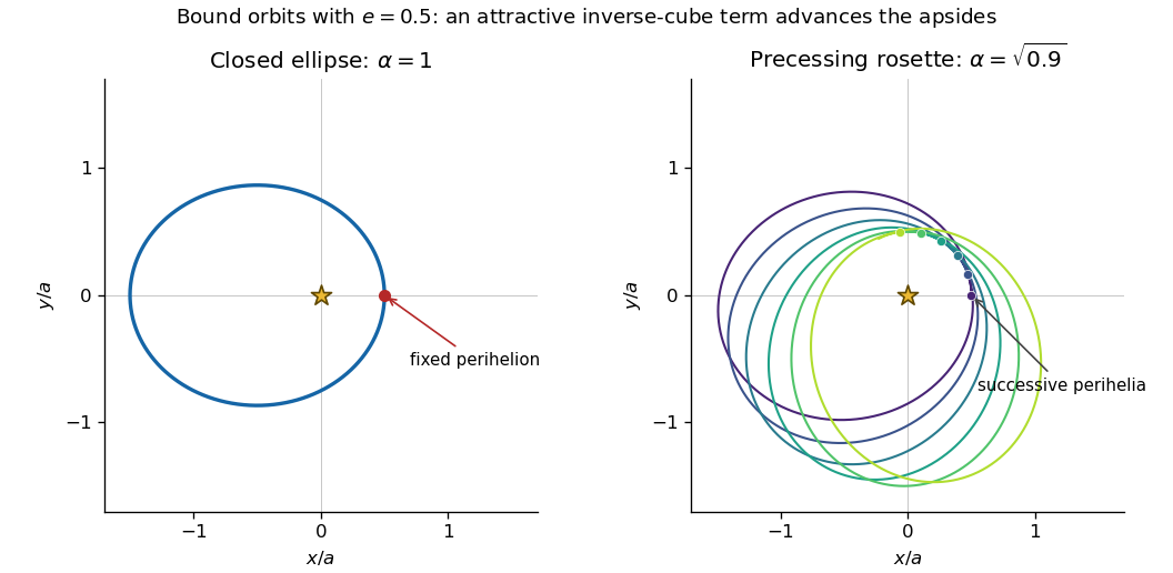
Closed Kepler ellipse and prograde precessing bound orbit under an attractive inverse-cube perturbation
. Details. 
The plotted precession is enlarged for visibility. Both examples have and the same turning radii; the second has .
For the precession rate, it is useful to derive the radial period rather than assume an unperturbed angular period. Set in the radial energy equation. On a complete radial cycle,Hence . Also and , so . For , inverse-cube perturbation of Kepler apsidal motion givesThere is a dimensional issue with the printed parameter: has units and has units , so has units . Retaining that definition literally, the requested expression isA dimensionless perturbation coefficient would instead be . In that convention the rate is . These two conventions must not be conflated.
Use the stated residual precession and period. The advance in one radial cycle isWith , the small-perturbation estimate becomesThe negative sign is required: an additional attractive inverse-cube acceleration advances perihelion, whereas the positive- term would make it regress. If a length-unit estimate of the printed is desired, and the solar value give through the radial-period law. ThusThe dimensionless value is the estimate obtainable directly from the supplied period, eccentricity and advance; the dimensional value additionally uses the solar gravitational parameter to set the length scale.
Articles by others on the same topic
There are currently no matching articles.