The common normal distribution for the child-specific random intercepts produces partial pooling. Children with little information borrow strength from the common population, while well-observed children retain more of their individual estimate. For fixed slopes and hyperparameters, let average the three responses after subtracting their slope terms. Multiplying the normal likelihood by the normal intercept prior distribution giveswith conditional variance . Thus small between-child variation produces stronger shrinkage towards . The common mean and variation are themselves learned from all children in this hierarchical Bayesian model.
Center the log-time predictor and the baseline log measurement near their sample means, so the intercept describes a typical predictor configuration. This reduces intercept-slope posterior correlation and can improve Markov chain Monte Carlo mixing. If exactly the original model is required, transform the intercept prior consistently when changing coordinates rather than silently assigning a different independent prior.
For weakly informed child effects, a non-centered Gaussian random-effect parameterization can also help:This retains the same conditional prior distribution for but removes its prior-scale dependence from the sampled . It can reduce strong dependence between the effects and . A centered parameterization can be better when each child's effect is very accurately observed, so improvement is not automatic. Blocking strongly correlated coefficients is another option. Check the resulting chains with Markov chain Monte Carlo convergence diagnostics and effective sample size of a Markov chain, rather than judging convergence from the number of iterations alone.
The bounded uniform prior distributions on the slopes and population intercept are proper and broad on their stated scale. They allow either sign but are not invariant to changes of units. The residual precision parameter has a proper shape-rate prior. Equivalently, has inverse-gamma distribution with the same shape and scale. This is a commonly used diffuse choice, but it is not literally noninformative and its tail behaviour merits sensitivity analysis.
The prior for is uniform on , so the induced density of isIt is integrable at zero, unlike the usual scale-invariant variance kernel . The latter kernel, often called the standard variance Jeffreys prior, would cause an improper posterior from a log-uniform random-effect scale prior here. After integrating the child intercepts, each child's response vector has a normal likelihood with covariance matrix . For fixed positive , this covariance remains nonsingular at , and the marginal likelihood has a positive finite limit there. On a compact set of the other parameters its positivity givesConsequently the scale-invariant kernel cannot be normalized to a posterior distribution. A proper prior on the standard deviation avoids this problem. This familiar scale prior is not necessarily the actual Jeffreys prior for an additive variance component derived from the observed-data likelihood; the latter can be finite at zero.
The baseline assay is a noisy measurement just like the follow-up assays. On the log scale, a normal distribution for its error is a reasonable approximation if variability is approximately multiplicative on the original titre scale. The latent represents the true baseline log-titre, withUsing a common variance is a simplifying assumption justified if baseline and follow-up measurements have comparable assay variability; it should not be treated as a fact guaranteed by the study design. Treating as exact ignores measurement error in a predictor and can lead to attenuation bias from classical measurement error and understated uncertainty.
Model 2 is an errors-in-variables model: the follow-up regression depends on a latent true baseline rather than substituting its noisy observation. A common normal distribution for the true baselines provides partial pooling and allows uncertainty about each baseline to propagate to the regression coefficients and predictions. Conditional on the shared parameters, the child-specific factorization isThe Directed acyclic graph below includes the shared parameters, the two local latent variables, both observed measurements, and the deterministic regression mean. The outer plate repeats over children and the inner plate over follow-up visits. Filled nodes are observed; rectangular mean nodes are deterministic.
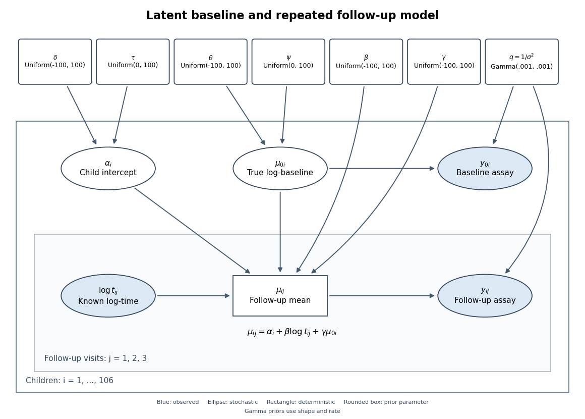
Directed graph of the latent-baseline random-intercept model, including shared priors, baseline measurement error and repeated follow-up visits
. Details. 
One complete adapted BUGS specification uses the non-centered form of the random intercept, retaining the original priors and adding proper broad priors for and :
for (i in 1:N) {
  z[i] ~ dnorm(0, 1)
  alpha[i] <- delta + tau*z[i]
  truebase[i] ~ dnorm(theta, baseprec)
  baseline[i] ~ dnorm(truebase[i], noiseprec)
  for (j in 1:3) {
    followmean[i,j] <- alpha[i] + beta*log(time[i,j]) + gamma*truebase[i]
    followup[i,j] ~ dnorm(followmean[i,j], noiseprec)
  }
}
noiseprec ~ dgamma(0.001, 0.001)
beta ~ dunif(-100, 100)
gamma ~ dunif(-100, 100)
delta ~ dunif(-100, 100)
tau ~ dunif(0, 100)
theta ~ dunif(-100, 100)
psi ~ dunif(0, 100)
baseprec <- 1/(psi*psi)
Here is the number of children,
baseline and followup contain the observed data, and dnorm uses precision rather than variance. The priors on the newly introduced population baseline mean and standard deviation are explicit choices, not consequences of the likelihood; sensible alternatives can be checked for sensitivity. The code uses the noisy baseline only in its own measurement likelihood, and uses truebase in every follow-up mean.The PDF output places inside the 95% credible interval for the time slope, whose endpoints are approximately and , and places inside the baseline slope interval, approximately to . Relative to their posterior standard deviations, the proposed fixed values are onlyfrom the posterior means. Thus the simpler choice is compatible with the fitted coefficient summaries and has a natural proportional-decay interpretation. It is a reasonable constrained model to compare, not proof of the exact equalities: separate marginal intervals do not establish a joint constraint, and a continuous posterior distribution assigns a specified point probability zero.
The reported Monte Carlo errors measure numerical uncertainty in the estimated posterior means, not uncertainty about the coefficients themselves. In particular, the baseline slope's Monte Carlo error is about 9% of its posterior standard deviation, appreciably larger than the corresponding proportion for the time slope. Longer or better-mixed chains may be needed for precise summaries.
The reported deviance information criterion differs byModel 3 has a mean Bayesian deviance worse by only , but its effective parameter count in DIC is lower by . The small fit cost is more than offset by the reduced complexity penalty, so the criterion gives a mild preference to Model 3. A difference this small should not be presented as decisive evidence, especially without the Monte Carlo error of the criterion difference.
The counts and are effective rather than literal parameter numbers. The likelihood includes child-specific intercepts and uncertain true baselines as well as global coefficients. With 106 of each local quantity and seven global parameters, Model 2 has 219 stochastic unknowns in a natural full representation, but partial pooling and other prior information reduce their effective contribution. Fixing two slopes lowers the effective count by about two, with a further small change from the fitted posterior. There is no reason for to be an integer, or to equal just the number of population-level regression coefficients.
For illustration, the deviances evaluated at posterior means implied by the table are for Model 2 and for Model 3. These differ from the average deviances because averaging a nonlinear deviance is not the same as evaluating it at an averaged parameter. This interpretation presumes the same observed-data likelihood convention in both fits; integrating local variables out before forming the deviance would define a different comparison. The DIC difference is not a Bayes factor.
Let denote the child's latent true baseline titre. With the constrained slopes, the conditional mean of log follow-up titre isExponentiating this log-scale center givesThus the conditional median, or geometric-mean titre, expressed as a fraction of true baseline titre, decays inversely with elapsed time; the child-specific intercept supplies the proportionality constant. It is not an exponential decay in time, and the formula is a follow-up model for , not an extrapolation to the immunisation instant .
For the arithmetic conditional mean, the lognormal distribution correction givesThe correction changes the constant but not the inverse-time dependence when the residual variance is constant. Averaging over random intercepts similarly preserves the time factor whenever the required expectation is finite.
Articles by others on the same topic
There are currently no matching articles.