If and , the prior odds on the null hypothesis areThese odds concern which model is true before seeing the observations. They are separate from the prior distribution of the success probability within the alternative model.
Use the orientation that favours the null hypothesis:For a composite model the denominator is its Bayesian model evidence, obtained by integrating the likelihood against the model's prior distribution. This Bayes factor exceeds one when the observed data have greater marginal probability under . By Bayes' theorem,Thus the posterior odds equal the prior odds multiplied by the Bayes factor. The reciprocal orientation instead gives .
Conditional on the success probability, the count has binomial distribution. Integrating its likelihood under the uniform prior distribution, or equivalently a beta distribution with parameters , givesThe prior predictive distribution is therefore uniform over the possible counts. Excluding the single point does not alter this integral because a continuous prior distribution gives that point zero probability. This calculation is the marginalization underlying Beta-binomial conjugacy.
Under the null hypothesis, , with expected value and variance . Approximating its probability at an integer by the normal distribution density over a unit-width cell givesDividing by the prior predictive distribution from the preceding part gives the uniform-alternative binomial Bayes factorThe second approximation replaces by . Both are large-sample approximations for counts in the central range, rather than exact identities at extreme counts.
The normal distribution standardized statistic for the binomial distribution count isBecause the alternative is two-sided, the approximate p-value is . A continuity correction replaces by and gives approximately , with the same conclusion. Thus the result is statistically significant at both the 5% and 1% levels. The p-value is a null tail probability, not a posterior probability that the null hypothesis is true.
Substituting the standardized deviation into the Bayes factor approximation givesThis is only a slight preference for the alternative, despite the small p-value. The two procedures measure different things: the p-value sums a tail under the null hypothesis, while the Bayes factor compares probabilities of the observed count under both models. The uniform alternative prior distribution spreads its probability over many success probabilities that fit the observations poorly. Only a narrow range around has large likelihood, and integrating over the whole alternative penalizes this diffuse prediction.
The prefactor makes the distinction especially clear. At a fixed standardized deviation , the p-value stays approximately , whereas eventually grows with . A fixed diffuse alternative can consequently favour the point null even while a conventional test rejects it. This is the same prior-width mechanism illustrated by the Jeffreys-Lindley paradox for a Gaussian point null.
An alternative that allows small departures from chance, while assigning little probability to near-perfect prediction or near-perfect failure, is more plausible than a uniform prior distribution. For example, a symmetric beta distribution with is centered at , withChoosing gives a prior standard deviation of about and concentrates on modest deviations. Its concentration should represent substantive beliefs specified before examining this experiment, rather than being tuned to the observed count. A continuous prior distribution centered at still places no point mass at ; the separate model prior probability supplies that mass.
No. A Bayes factor favouring the alternative means , but the posterior odds are . They are less than one only if . For example, prior odds of on the null hypothesis, combined with a Bayes factor of in favour of the alternative, still give posterior odds of on the null hypothesis. An unusual claim can require substantial evidence to overcome low initial plausibility.
Take the exposure as known and positive. The Poisson distribution log-likelihood, up to a parameter-independent constant, is . Its first two derivatives areSince , the Fisher information isThe Jeffreys prior is proportional to its square root. Removing the constant givesThis is an improper prior: its integral diverges at infinity.
Multiplying the Poisson distribution likelihood by the Jeffreys prior gives the posterior density kernelThus, in shape-rate convention,It is a proper posterior distribution even when , provided . The posterior mean and posterior variance are and . This is Poisson-gamma conjugacy with unequal exposures, with the zero-rate prior interpreted as an improper kernel.
A proper gamma approximation to a Poisson Jeffreys prior uses shape and a small positive rate :Its density is proportional to , so where is small its kernel approximates the Jeffreys prior. After observing the data, Poisson-gamma conjugacy gives , which converges to the preceding posterior distribution as . This is an approximation of an improper kernel on the relevant parameter range, not a weak limit to a normalized Jeffreys probability distribution. The shape must be ; a small-shape gamma prior would approximate a different power of .
Under independent area counts and independent area prior distributions, the joint posterior distribution factors into the gamma posteriors. For each simulation , draw one joint vector by independently generatingRank the risks within that joint draw, taking rank one to mean highest risk:The empirical posterior rank distribution and highest-risk probability areIndependent gamma draws make this direct Monte Carlo integration, so Markov chain Monte Carlo is unnecessary here. Continuous posteriors give ties probability zero, and the highest-risk probabilities sum to one. The same ranking calculation can be applied to dependent joint draws from a richer hierarchical Bayesian model; ranking separate posterior means would discard the uncertainty that the program is intended to measure.
For a shape-rate gamma distribution , the mean and variance conditions requireThe first equation gives , and the second then gives . HenceThis proper prior distribution is centered on the national reference risk, while allowing genuine between-area variation.
The new prior density contributes the factor . Multiplication by the Poisson distribution likelihood givesIts posterior mean displays the resulting shrinkage:The observed risk ratio is pulled towards one, most strongly for small exposures. The posterior variance is .
The informative gamma distribution prior distribution discourages extreme risks caused by small denominators. Its influence is strongest where the exposure is small, while large-exposure areas are predominantly determined by their likelihood. Consequently an area previously appearing near the top because of a noisy high raw risk ratio may have its highest-risk probability reduced, and the posterior rank distributions of poorly observed areas tend to overlap more rather than suggesting a precise league table.
There is no universal claim that every rank distribution becomes wider or narrower: unequal exposures produce unequal shrinkage and can change the ordering, while the new prior also changes the uncertainty in the risks. In the limiting case of negligible information for every area, all area posteriors approach the same independent continuous prior distribution. Symmetry then gives each area probability of occupying each rank. This illustrates why modest differences between weakly observed areas should not yield confident rankings.
The posterior probability answers a natural directional question: how likely is this area's risk to exceed the reference risk? It accounts for uncertainty rather than declaring an increase from the point estimate alone. However, it does not distinguish a negligible increase from a clinically important one, and it combines prior beliefs with evidence from the data. With an informative prior distribution, a large probability may already have been present before observation, or a genuinely surprising count may be strongly moderated by the prior.
To measure the evidence supplied by the observations, compare posterior and prior odds. If under the chosen proper prior distribution, the Bayes factor for increased versus nonincreased risk isThis follows from the posterior odds identity when the two models use the original prior conditioned respectively on and . For the specified prior, is the upper tail at one of ; centering its mean at one does not make this tail probability exactly . To address seriousness itself, choose a substantive excess and report the posterior probability of , together with an interval for the size of the excess. An evidence ratio and a meaningful risk threshold answer different, complementary questions.
The logarithm is strictly increasing, so maximizing the likelihood function is equivalent to maximizing its logarithm. Multiplication by reverses that ordering. Thus, whenever the maximum is attained,Here the Bayesian deviance includes the likelihood constants. Parameter-independent constants do not alter the minimizer, but a common convention must be retained when comparing criteria between models.
Under the usual regular, identifiable, fixed-dimensional setting, the maximum-likelihood estimator is an interior point with vanishing log-likelihood gradient, and the observed information is positive definite. DefineThe second-order Taylor expansion of the Bayesian deviance isWith a prior density approximately constant over the likelihood's concentration region, the posterior density is therefore proportional toRecognizing the multivariate normal density givesTypically grows at rate and the posterior concentrates in a region of radius , making higher-order terms negligible under the regularity assumptions. The local flatness assumption concerns this region, not necessarily the entire parameter space. Boundary maxima, unidentified directions, or persistent multiple modes can invalidate this approximation.
Conditional on the observed data, the preceding multivariate normal distribution approximation implies thatThe deviance expansion consequently givesThe sum of squares of independent standard normal distribution variables has chi-squared distribution with degrees of freedom. Hence, as a statement about the posterior distribution of the Bayesian deviance,The data are fixed here and the parameter varies according to its posterior; this is not a claim about resampling the data.
Let and . The usual effective parameter count in DIC isWith the locally flat prior distribution, and the mean of the chi-squared distribution excess is . Thus , while , giving .
More generally, the quadratic posterior deviance moments give the effective count. Within the same approximation, let the posterior covariance matrix be . The expectation of a quadratic form giveswhereas evaluation at omits the trace term. Therefore . For a flat prior, and the trace is ; informative prior shrinkage can reduce this effective count.
Using the same Bayesian deviance convention, the deviance information criterion and Akaike information criterion areBoth combine a lack-of-fit term with a complexity penalty; smaller values are preferred among comparable models. Under the locally flat prior distribution and the regular multivariate normal distribution approximation, and , soAll fitted parameters counted in the likelihood, including unknown dispersion parameters, belong in . The equivalence need not hold for informative priors, nonregular models, or different choices of the likelihood's latent-variable representation.
For retained Markov chain Monte Carlo draws , calculate both the parameter average and the average deviance . Two estimates areThe first uses the approximate equality of the posterior mean and maximum-likelihood estimator. The second subtracts the mean of the chi-squared distribution deviance excess. These are different operations: evaluation after averaging versus averaging after evaluation. Both rely on a well-mixed chain and the regular locally flat-prior approximation. The smallest sampled deviance is an upper bound on the true minimum, but merely taking that minimum can be inefficient in high dimension because few draws approach the mode closely.
The alternative effective count isUnder the locally flat-prior approximation, the constant contributes no variance, and the remaining chi-squared distribution term has variance . Hence , the same calibration as the usual effective parameter count in DIC. It can be estimated by half the sample variance of deviance draws, without evaluating deviance at a parameter average.
This is a calibrated alternative, not a general identity with . For example, with a quadratic deviance and a multivariate normal distribution posterior of mean and covariance , putting givesThey agree when and , but informative priors can change both the covariance and the displacement of the posterior mean. Their equality should therefore not be assumed outside the stated regime.
The common normal distribution for the child-specific random intercepts produces partial pooling. Children with little information borrow strength from the common population, while well-observed children retain more of their individual estimate. For fixed slopes and hyperparameters, let average the three responses after subtracting their slope terms. Multiplying the normal likelihood by the normal intercept prior distribution giveswith conditional variance . Thus small between-child variation produces stronger shrinkage towards . The common mean and variation are themselves learned from all children in this hierarchical Bayesian model.
Center the log-time predictor and the baseline log measurement near their sample means, so the intercept describes a typical predictor configuration. This reduces intercept-slope posterior correlation and can improve Markov chain Monte Carlo mixing. If exactly the original model is required, transform the intercept prior consistently when changing coordinates rather than silently assigning a different independent prior.
For weakly informed child effects, a non-centered Gaussian random-effect parameterization can also help:This retains the same conditional prior distribution for but removes its prior-scale dependence from the sampled . It can reduce strong dependence between the effects and . A centered parameterization can be better when each child's effect is very accurately observed, so improvement is not automatic. Blocking strongly correlated coefficients is another option. Check the resulting chains with Markov chain Monte Carlo convergence diagnostics and effective sample size of a Markov chain, rather than judging convergence from the number of iterations alone.
The bounded uniform prior distributions on the slopes and population intercept are proper and broad on their stated scale. They allow either sign but are not invariant to changes of units. The residual precision parameter has a proper shape-rate prior. Equivalently, has inverse-gamma distribution with the same shape and scale. This is a commonly used diffuse choice, but it is not literally noninformative and its tail behaviour merits sensitivity analysis.
The prior for is uniform on , so the induced density of isIt is integrable at zero, unlike the usual scale-invariant variance kernel . The latter kernel, often called the standard variance Jeffreys prior, would cause an improper posterior from a log-uniform random-effect scale prior here. After integrating the child intercepts, each child's response vector has a normal likelihood with covariance matrix . For fixed positive , this covariance remains nonsingular at , and the marginal likelihood has a positive finite limit there. On a compact set of the other parameters its positivity givesConsequently the scale-invariant kernel cannot be normalized to a posterior distribution. A proper prior on the standard deviation avoids this problem. This familiar scale prior is not necessarily the actual Jeffreys prior for an additive variance component derived from the observed-data likelihood; the latter can be finite at zero.
The baseline assay is a noisy measurement just like the follow-up assays. On the log scale, a normal distribution for its error is a reasonable approximation if variability is approximately multiplicative on the original titre scale. The latent represents the true baseline log-titre, withUsing a common variance is a simplifying assumption justified if baseline and follow-up measurements have comparable assay variability; it should not be treated as a fact guaranteed by the study design. Treating as exact ignores measurement error in a predictor and can lead to attenuation bias from classical measurement error and understated uncertainty.
Model 2 is an errors-in-variables model: the follow-up regression depends on a latent true baseline rather than substituting its noisy observation. A common normal distribution for the true baselines provides partial pooling and allows uncertainty about each baseline to propagate to the regression coefficients and predictions. Conditional on the shared parameters, the child-specific factorization isThe Directed acyclic graph below includes the shared parameters, the two local latent variables, both observed measurements, and the deterministic regression mean. The outer plate repeats over children and the inner plate over follow-up visits. Filled nodes are observed; rectangular mean nodes are deterministic.
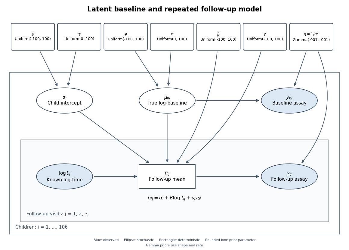
Directed graph of the latent-baseline random-intercept model, including shared priors, baseline measurement error and repeated follow-up visits
. Details. 
One complete adapted BUGS specification uses the non-centered form of the random intercept, retaining the original priors and adding proper broad priors for and :
for (i in 1:N) {
  z[i] ~ dnorm(0, 1)
  alpha[i] <- delta + tau*z[i]
  truebase[i] ~ dnorm(theta, baseprec)
  baseline[i] ~ dnorm(truebase[i], noiseprec)
  for (j in 1:3) {
    followmean[i,j] <- alpha[i] + beta*log(time[i,j]) + gamma*truebase[i]
    followup[i,j] ~ dnorm(followmean[i,j], noiseprec)
  }
}
noiseprec ~ dgamma(0.001, 0.001)
beta ~ dunif(-100, 100)
gamma ~ dunif(-100, 100)
delta ~ dunif(-100, 100)
tau ~ dunif(0, 100)
theta ~ dunif(-100, 100)
psi ~ dunif(0, 100)
baseprec <- 1/(psi*psi)
Here is the number of children,
baseline and followup contain the observed data, and dnorm uses precision rather than variance. The priors on the newly introduced population baseline mean and standard deviation are explicit choices, not consequences of the likelihood; sensible alternatives can be checked for sensitivity. The code uses the noisy baseline only in its own measurement likelihood, and uses truebase in every follow-up mean.The PDF output places inside the 95% credible interval for the time slope, whose endpoints are approximately and , and places inside the baseline slope interval, approximately to . Relative to their posterior standard deviations, the proposed fixed values are onlyfrom the posterior means. Thus the simpler choice is compatible with the fitted coefficient summaries and has a natural proportional-decay interpretation. It is a reasonable constrained model to compare, not proof of the exact equalities: separate marginal intervals do not establish a joint constraint, and a continuous posterior distribution assigns a specified point probability zero.
The reported Monte Carlo errors measure numerical uncertainty in the estimated posterior means, not uncertainty about the coefficients themselves. In particular, the baseline slope's Monte Carlo error is about 9% of its posterior standard deviation, appreciably larger than the corresponding proportion for the time slope. Longer or better-mixed chains may be needed for precise summaries.
The reported deviance information criterion differs byModel 3 has a mean Bayesian deviance worse by only , but its effective parameter count in DIC is lower by . The small fit cost is more than offset by the reduced complexity penalty, so the criterion gives a mild preference to Model 3. A difference this small should not be presented as decisive evidence, especially without the Monte Carlo error of the criterion difference.
The counts and are effective rather than literal parameter numbers. The likelihood includes child-specific intercepts and uncertain true baselines as well as global coefficients. With 106 of each local quantity and seven global parameters, Model 2 has 219 stochastic unknowns in a natural full representation, but partial pooling and other prior information reduce their effective contribution. Fixing two slopes lowers the effective count by about two, with a further small change from the fitted posterior. There is no reason for to be an integer, or to equal just the number of population-level regression coefficients.
For illustration, the deviances evaluated at posterior means implied by the table are for Model 2 and for Model 3. These differ from the average deviances because averaging a nonlinear deviance is not the same as evaluating it at an averaged parameter. This interpretation presumes the same observed-data likelihood convention in both fits; integrating local variables out before forming the deviance would define a different comparison. The DIC difference is not a Bayes factor.
Let denote the child's latent true baseline titre. With the constrained slopes, the conditional mean of log follow-up titre isExponentiating this log-scale center givesThus the conditional median, or geometric-mean titre, expressed as a fraction of true baseline titre, decays inversely with elapsed time; the child-specific intercept supplies the proportionality constant. It is not an exponential decay in time, and the formula is a follow-up model for , not an extrapolation to the immunisation instant .
For the arithmetic conditional mean, the lognormal distribution correction givesThe correction changes the constant but not the inverse-time dependence when the residual variance is constant. Averaging over random intercepts similarly preserves the time factor whenever the required expectation is finite.
Articles by others on the same topic
There are currently no matching articles.