Past exam of the mathematics course of the University of Cambridge / 2012 / iii / Paper 50 (Advanced Quantum Field Theory)

Set $\Delta =T/M$, $q_0=q$, and $q_M=q^{\prime }$. The Trotter product formula separates the kinetic and potential energy evolution to first order in $\Delta$. Inserting $M-1$ resolutions of the identity in the position operator basis and using the free short-time kernel givesThe exponent converges formally to the action along the path. The prefactors and intermediate integrations define the time-sliced configuration-space path integral measure, soA real-time path integral is an oscillatory limit with the Feynman i-epsilon prescription, rather than an ordinary probability integral. The operator derivation assumes the usual self-adjointness and product-formula hypotheses for the Hamiltonian.

For a quadratic potential energy write $q=q_c+\eta$, with $\eta (0)=\eta (T)=0$ and ${\ddot{q}}_c+V^{\prime }(q_c)=0$. The first variation vanishes by the Euler-Lagrange equation and the fixed endpoints. Because $V$ is quadratic, the remaining expansion is exact:Here integration by parts has no boundary contribution. Translation of the integration variables leaves the time-sliced measure unchanged. Thus the Gaussian path integral over $\eta$ is independent of the endpoint values, and the entire endpoint dependence lies in $e^{iS[q_c]}$.

Expanding $\eta$ in eigenfunctions satisfying Dirichlet boundary conditions, each real mode contributes an inverse square root of its quadratic eigenvalue, with the oscillatory phase fixed by continuation. Normalizing against $A_0={\partial }_t^2$ gives a precise determinant-ratio form:The determinant ratio is meaningful after a common regulator; the phase is part of the prescription. It is equivalent to writing $N=C(T)({\det }_{D}A{)}^{-1/2}$ with an endpoint-independent normalization.

For example, if $V^{\prime \prime }={\omega }^2$, the Dirichlet oscillator determinant ratio isA linear or constant term in $V$ changes the action but not this prefactor. The formula holds away from conjugate times, when the boundary problem and determinant are nonsingular. At $\sin \omega T=0$, it must be continued as a distribution with its Maslov index phase; the assertion of an ordinary finite prefactor cannot be used literally there. For the unshifted oscillator, at $T=r\pi /\omega$ the kernel is $e^{-ir\pi /2}\delta (q^{\prime }-(-1{)}^{r}q)$.

For the full-line source integral, impose vacuum boundary conditions by adiabatic damping. Take the source initially as a test function, so its pairings with the Green function are defined. After integration by parts, writeWith the Fourier transform convention $G(t)=\int d\omega e^{i\omega t}\tilde{G}(\omega )/(2\pi )$, the inverse isSet $q=\eta -GJ$. Completing the square givesand consequentlyThe Gaussian functional integral $Z[0]$ is source independent and contains the regulated determinant. This is most naturally read as a normalized vacuum generating functional. For $m>0$, closing the frequency contour gives $G(t)=-i{e}^{-im|t|}/(2m)$; the time-ordered oscillator two-point function is $iG(t)$. This checks the sign of the source exponent and identifies the required vacuum prescription.

Use the metric signature $(-,+,\dots ,+)$, so $p^2=-p_0^2+{\mathbf{p}}^2$, and the weight $e^{iS}$. The momentum-space Feynman rules for the massless Phi-fourth theory are: an internal scalar line contributes $-i/(k^2-iϵ)$; a quartic interaction vertex contributes $-i\lambda$ with its momentum-conservation delta function; every independent loop is integrated with $d^{d}k/(2\pi {)}^d$; and each graph is multiplied by its Feynman-diagram symmetry factor. All external momenta can be taken incoming. These rules follow by expanding the interaction exponential and contracting free fields with the Wick theorem.

For a connected graph with $I$ internal lines, $V$ interaction vertices and $L$ loops,Here $D$ is the superficial degree of divergence. In four dimensions,Odd $n$ vanish by Z2 symmetry. Thus only the nonvacuum two-point and four-point one-particle-irreducible Feynman diagrams can have overall ultraviolet divergences: degree two for $n=2$, degree zero for $n=4$. Vacuum graphs with $n=0$ may also diverge but cancel from normalized correlators. This is an overall power-counting statement; subgraphs must be subtracted before using it to conclude finiteness for $n\ge 6$.

For the full one-particle-irreducible vertices, the tree-level quadratic kernel and quartic interaction giveIf ${\hat{\tau }}_2$ is instead reserved for interaction-generated self-energy insertions, its tree value is zero and $-p^2$ is displayed separately as the free inverse kernel. The distinction is only that convention; the loop insertions below are unchanged.

The requested one-loop diagrams are the two-point tadpole diagram and the three four-point bubble diagrams. Each has symmetry factor $1/2$. The three bubble channels correspond to $P_s=p_1+p_2$, $P_t=p_1+p_3$, $P_u=p_1+p_4$.

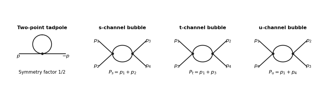
The tadpole insertion obeysIn massless dimensional regularization this scaleless integral is zero. A mass or cutoff regulator exposes the ultraviolet divergence allowed by power counting; its vanishing in the scaleless convention does not remove the need to include this diagram.

For a bubble, the vertex and quantum field theory propagator factors give $(-i\lambda {)}^2(-i{)}^2/2={\lambda }^2/2$. The PDF defines $f$ with the factor $1/i$ outside the Minkowski integral, so the integral itself is $if(P^2)$. ThereforeThe converted TeX misplaces this $i$ as though it were part of the exponent of $(2\pi )$; keeping the printed $1/i$ is essential to this real pole coefficient.

For nonexceptional Euclidean external momentum, Wick rotation cancels that factor $1/i$. Use a Feynman parameter and translate the integration variable:For example, represent the inverse square as ${\int }_0^{\infty }d\alpha \alpha e^{-\alpha ({\ell }^2+\Delta )}$, do the Gaussian momentum integral, and then use the Gamma function. This also derives the formula rather than assuming a loop-integration table. At $d=4-\epsilon$, $\Gamma (\epsilon /2)=2/\epsilon +O(1)$ and the parameter integral tends to one, givingTake $P^2>0$ before continuation back to Minkowski momenta. At $P=0$, a massless scaleless integral mixes ultraviolet and infrared issues, so it cannot be used to read off this pole.

Introduce a renormalization scale $\mu$ and a quartic counterterm. With $\lambda$ denoting a dimensionless renormalized coupling constant,After factoring out ${\mu }^{\epsilon }$ from the vertex, each loop contains ${\mu }^{\epsilon }{f}_d$. The counterterm contributes $-\delta \lambda$ to ${\hat{\tau }}_4$ and cancels the pole from all three channels. More explicitly,In modified minimal subtraction, replace the pole-only counterterm bywhich subtracts the first three terms inside the brackets. The finite renormalized quartic scalar vertex is thenAnother renormalization condition can change the finite constant, but not the pole cancellation or the momentum-dependent logarithms. The corresponding timelike expressions follow by the same Feynman continuation.

Loop integrals require a subtraction prescription. Even when the classical coupling constant is dimensionless and there is no mass, specifying its renormalized value means specifying a momentum or length scale at which it is measured. Dimensionless logarithms then involve that renormalization scale $\mu$. Changing $\mu$ changes the renormalized coupling constant and wave-function renormalization while leaving bare quantities fixed. In a theory whose renormalization-group beta function and anomalous dimension both vanish, this scale dependence may disappear; the generic statement concerns the interacting renormalized theory.

Write ${\varphi }_B=Z_{\varphi }^{1/2}{\varphi }_R$ and $G_{n,R}=Z_{\varphi }^{-n/2}{G}_{n,B}$. DefineBare correlation functions do not depend on the arbitrary subtraction scale. Differentiating their relation to renormalized correlation functions gives the Callan-Symanzik equationIt expresses the compensation between explicit scale dependence, running coupling and wave-function renormalization. In this convention the field scaling dimension is its engineering dimension plus ${\gamma }_{\varphi }$ at a fixed point; the critical-exponent notation $\eta$ often used for the anomalous dimension equals $2{\gamma }_{\varphi }$.

A renormalization-group fixed point satisfies $\beta (g_{\ast })=0$. It is ultraviolet attractive if the flow approaches it as $\mu \to \infty$, and infrared attractive if the flow approaches it as $\mu \to 0$. For a simple isolated zero, $\delta g\propto {\mu }^{{\beta }^{\prime }(g_{\ast })}$: a negative derivative gives ultraviolet attraction, a positive derivative infrared attraction. Marginal zeros, such as a cubic renormalization-group beta function at the origin, require looking at the first nonzero nonlinear term.

Put $z=p^2/{\mu }^2>0$, $t=\frac{1}{2}\log z$, and write the dimensionless quantum field theory propagator factor as $d(z,g)$. The two-point Callan-Symanzik equation becomesLet $\bar{g}(0)=g$ and $d\bar{g}/dt=\beta (\bar{g})$. The renormalization-group characteristic solution for a two-point function isWhere $\beta \ne 0$, the exponent is $2{\int }_g^{\bar{g}(t)}{\gamma }_{\varphi }(u)/\beta (u)du$. Thus the ultraviolet behavior depends on where the running coupling goes and on the anomalous dimension accumulated along the flow. A weak ultraviolet fixed point or asymptotically free limit permits perturbative evaluation; a flow to large values of the coupling constant does not.

For $\beta (g)=-b{g}^3$ and ${\gamma }_{\varphi }=c{g}^2$, $b>0$,ConsequentlyFor large positive $z$, the coupling constant tends to zero. If the normalization function $d(1,g)$ has a finite nonzero free-field limit $d(1,0)$, then $d(z,g)\sim d(1,0)[b{g}^2\log z{]}^{c/b}$. Equivalently, with $\Lambda =\mu \exp [-1/(2b{g}^2)]$,The positive exponent follows from the sign of $+n{\gamma }_{\varphi }$ in the printed RG equation; changing the field-renormalization anomalous dimension convention would change both signs together.

For the quintic renormalization-group beta function, set $B=-b>0$ and rename its positive quintic coefficient $A$ to avoid confusion with the later gauge-theory coupling constant. Then $\beta (g)=g^3(B-A{g}^2)$ has a nonzero fixed pointEvery nonzero positive running coupling in the perturbative basin approaches this ultraviolet fixed point, rather than approaching zero. The zero coupling constant is infrared attractive. If the same ${\gamma }_{\varphi }=c{g}^2$ is retained, the large-momentum factor is $d(z,g)\sim C{z}^{cB/A}$, assuming a regular nonzero matching factor at the fixed point. More generally the exponent is ${\gamma }_{\varphi }(g_{\ast })$. A fixed point at a large coupling constant inferred from a truncated renormalization-group beta function is only a formal extrapolation; perturbative control requires $B/A$ small.

For the gauge theory use the supplied convention $a=g^2/(16{\pi }^2)$ and evolution variable $L=\log {\mu }^2$. Asymptotic freedom requires ${\beta }_0>0$, or $n<11N/2$. To one-loop accuracy,The integration constant $\Lambda$ is an example of dimensional transmutation. With two loops this is the leading asymptotic expression, not an exact equality: if $\mathcal{L}=\log ({\mu }^2/{\Lambda }^2)$ is large,The expansion presumes fixed coefficients and a scale high enough to enter the ultraviolet regime.

Choose $n=11N/2-\delta$ with $0<\delta \ll N$, respecting integer flavor counts. The supplied coefficients becomeThus ${\beta }_1<0$ for sufficiently small $\delta /N$, and the two-loop flow has the Banks-Zaks fixed pointBoth $a_{\ast }$ and the loop-counting combination $N{a}_{\ast }$ are small. Its slope is ${\beta }^{\prime }(a_{\ast })=-{\beta }_0^2/{\beta }_1>0$, so it is infrared attractive. For even large $N$, taking $n=11N/2-1$ provides an explicit integer sequence with the desired parametric hierarchy. As a finite example, $N=3,n=16$ gives ${\beta }_0=1/3$, ${\beta }_1=-302/3$ and $a_{\ast }=1/302$. The fermion-count convention is the one encoded by the given coefficients.

For adjoint-valued quantities write $(X\times Y{)}_a={\epsilon }_{abc}{X}_b{Y}_c$. Substituting the infinitesimal transformation into the gauge field strength and using the Jacobi identity givesA useful way to organize the calculation is $[D_{\mu },D_{\nu }]X=g{F}_{\mu \nu }\times X$: the gauge field strength transforms covariantly because the gauge covariant derivative does. Thus $\delta (F_a^{\mu \nu }{F}_{\mu \nu a})=2g{F}_a^{\mu \nu }{\epsilon }_{abc}{F}_{\mu \nu b}{\lambda }_c=0$ by antisymmetry. This proves gauge invariance of the Yang-Mills action.

The Yang-Mills equations are $D_{\mu }{F}^{\mu \nu }=0$. They determine physical evolution only modulo gauge redundancy: gauge transformations with arbitrary spacetime-dependent parameters take solutions to equivalent solutions. In Hamiltonian mechanics, $A_0$ has no independent quadratic time-derivative term, and the corresponding equation is a Gauss law constraint in gauge theory. A gauge parameter can vanish with its necessary derivatives on the initial slice yet change the later potential energy, so the potential energy itself is not uniquely fixed by initial physical data.

In the uncorrected path integral, integration along gauge orbits overcounts equivalent fields. At the perturbative level the quadratic operator of the kinetic term has gauge zero modes and no inverse, so it does not supply a quantum field theory propagator. Gauge fixing together with the Faddeev-Popov determinant removes this obstruction in the local perturbative construction.

For the odd BRST transformation, products obey the graded Leibniz rule. The adjoint product with Grassmann variables satisfiesIn particular, $c\times c$ is not zero, and $c\times Dc=Dc\times c$. The supplied transformations givesince the even covariant derivative obeys $D(c\times c)=2(Dc)\times c$. For the ghost,The final equality is the graded Jacobi identity; in components it is the Jacobi identity for ${\epsilon }_{abc}$ contracted with the totally antisymmetric product of three ghosts. Also $s^2\bar{c}=-sb=0$ and $s^{2}b=0$. The square of an odd derivation is an even derivation, because its two mixed product terms cancel. Hence $s^2=0$ on every polynomial in the fields, off shell, without imposing field equations.

Let $\Psi =\int d^{d}x[{\partial }^{\mu }{\bar{c}}_a{A}_{\mu a}+\xi {\bar{c}}_a{b}_a/2]$ be the gauge-fixing fermion. Since $sF=gF\times c$, $s{\mathcal{L}}_{\mathrm{YM}}=0$. The BRST-exact operator in ${\mathcal{L}}_q={\mathcal{L}}_{\mathrm{YM}}-s\psi$ has zero variation by BRST nilpotence, soTo see the resulting kinetic terms and signs, expand the exact term with $s\bar{c}=-b$:After integration by parts,The auxiliary Nakanishi-Lautrup field $b$ can be completed into a square and integrated out, giving the gauge-fixing term $-(\partial \cdot A_a{)}^2/(2\xi )$ for $\xi \ne 0$. At $\xi =0$, retain $b$ as the multiplier enforcing the gauge condition rather than divide by $\xi$. The Grassmann Gaussian integral gives the determinant of the gauge-condition operator $-\partial \cdot D$. Field-independent normalizations cancel in the normalized integral; insertions involving $b$ can be handled before integration or through its source terms.

At $g=0$ the gauge-fixed quadratic operator is invertible with the usual prescription, and the ghosts have a quadratic kinetic term. The remaining terms are cubic gauge interactions of order $g$, quartic gauge interactions of order $g^2$, and a ghost-gauge interaction of order $g$. Expanding them and using Wick contractions gives a perturbative expansion for any defined polynomial insertion $X$ of the fields. The exponent is the gauge-fixed action $S_q$, as printed in the PDF; the converted TeX incorrectly substitutes $S_A$.

At $\xi =1$, the free gauge action, up to a boundary term, is $\frac{1}{2}\int A_{\mu a}\square A_a^{\mu }$. Its Fourier kernel is $-p^2{\eta }_{\mu \nu }{\delta }_{ab}$. With the mostly-plus convention used above, the Feynman-gauge adjoint propagator isThis is consistent with the scalar-line convention in Question 2.

Finally define the odd functional $B=\frac{1}{2}\int d^{d}x{\bar{c}}_a{b}_a$. Then ${\partial }_{\xi }{S}_q=-sB$. Differentiating the normalized expectation, including its denominator, givesfor an insertion with no explicit $\xi$ dependence. A physical gauge-invariant insertion $X[A]$ is BRST-closed, since its infinitesimal gauge variation vanishes also when the parameter is replaced by $c$. The assumed BRST Ward identity gives $⟨sB⟩=0$ and $⟨s(XB)⟩=0$. For an even $X$ with $sX=0$, the latter says $⟨XsB⟩=0$. ThereforeThe same conclusion holds for any BRST-closed insertion. Mere color-singlet invariance of an arbitrary ghost-dependent expression need not imply $sX=0$; the physical-observable qualification is essential. The proof uses the invariant-measure assumptions encoded in the stated Ward identity.