An oil spill under sea ice first reaches the underside through buoyancy. Oil droplets and gas bubbles rise relative to the surrounding water; their collective buoyancy drives an entraining buoyant plume, while ocean currents bend the plume and carry small droplets away. Droplet size matters: small droplets rise slowly and can be dispersed or partly dissolved before arriving, whereas coalescence produces faster-rising drops. Gas expansion, dissolution and the ambient density stratification change the plume on its ascent. Consequently the arrival footprint can be displaced from the well, and the oil arrival rate at the ice need not equal the discharge rate at the seabed.
The combinations of cover and motion give four distinct collection geometries. Each must then be combined with the four age-and-relief cases below; this accounts for all sixteen combinations without treating age as a substitute for geometry.
- Under continuous fast ice, the receiving underside stays near the source. Oil accumulates locally, spreads laterally along the ice–water interface and can fill successively higher buoyant traps. Currents can still transport it beneath the stationary cover.
- Under continuous moving sea ice, different parts of the underside cross the arrival footprint. Oil adhering to, or trapped beneath, an ice floe is exported with it; oil remaining mobile relative to the ice is also transported by currents. The balance of arrival and the fresh underside passing the source determines whether deposition is continuous.
- With broken but anchored fast ice, oil can collect beneath separate stationary pieces, escape around their edges into leads, or encounter another piece downstream. The exposed water allows evaporation and wave-driven dispersion that are restricted beneath an unbroken cover. Here “fast” means anchored pieces, rather than freely drifting fragments.
- With broken moving ice floes, there is both intermittent capture by passing floes and intermittent direct surfacing in the gaps. Collisions, overturning and changing leads redistribute oil between undersides, floe edges and open water; the contaminated floes can travel far from the discharge.
For each of these four geometries, the age-and-relief combinations have the following effects.
- Smooth first-year sea ice supports a thin spreading lens. Its saline pore network can later provide a route into the ice when connected brine channels open; a cold, poorly connected network can initially exclude oil.
- Deformed first-year sea ice has upward recesses, ridge keels and rubble interstices that partition the lens into reservoirs. Locally much thicker oil can be stored, and liquid-filled interstices can provide routes into a ridge. The available connected storage volume matters more than the flat-interface lens thickness.
- Smooth multi-year sea ice still obeys the flat-interface capillary balance wherever the receiving surface is flat. Its previous drainage and melt history changes pore salinity and connected pathways, so its incorporation behaviour need not match saline young ice.
- Deformed multi-year sea ice combines old ridge and melt topography with a repeatedly modified pore structure. Oil can be retained in deep underside pockets and redistributed when the floe melts, cracks or overturns. Neither age class is invariably more permeable: temperature, liquid fraction and connectivity control the permeability of a porous medium.
Thus deformation increases local storage in either age class; motion changes residence time and export in either geometry; and gaps permit direct surfacing in either stationary or moving ice. These distinctions remain important even when two covers have the same mean thickness.
During growth, new sea ice can form around the edges of a lens or at available water-contacting surfaces and enclose oil between successive layers. Oil interrupts direct ice–water contact and changes thermal resistance, so incorporation is not simply freezing a pure oil layer. Oil droplets can be caught in a growing skeletal layer, and connected brine channels allow upward migration when buoyancy overcomes capillary entry resistance. In spring, warming increases the liquid fraction and opens pathways; meltwater and brine circulation can redistribute oil internally. Oil can then reach the surface and melt ponds, darken the ice, or be released to open water when the enclosing ice disappears. Thick ridge pockets may survive longer than flat lenses. The coupling between brine drainage, warming and oil migration is documented by field observations of oil entrainment in first-year ice.
A shorter freezing season gives less time for encapsulation and long-term storage. Less multi-year sea ice, greater open-water exposure and earlier breakup shift more of the spill into surface slicks and mobile fragments. Earlier warming can release stored oil sooner, while reduced cover permits more wave mixing and evaporation. This does not guarantee rapid removal: a plume may still encounter fast ice or deformed reservoirs, and oil-induced darkening promotes ice-albedo feedback. These changes alter exposure, transport and recovery opportunities rather than making every warming effect favourable.
For the oil lens capillary balance, distinguish the three interfacial tensions , and , where the subscripts denote ice, oil and water. Replacing an ice–water area by an ice–oil and oil–water pair costs the effective interfacial energyFor a broad, shallow, non-wetting lens of volume , neglect the small edge region. The interfacial energy is . Because oil is lighter than water, moving it downward through a depth costs buoyancy potential energy . At fixed their sum isSetting givesThe second derivative is positive when . Equivalently, if is the contact angle measured through the oil, the contact-line balance gives , so . These are the interfacial quantities required, rather than alone. If , complete wetting replaces this finite-lens balance; if the ice is rough, pocket geometry replaces the flat-lens approximation. oil–ice–water interfacial experiments give the corresponding contact-angle description.
The printed numerical premise is defective. A crude-oil density near means , rather than the printed . Moreover, the specified oil–ice tension does not specify . Even if were assumed to be , taking would give with the literal density and with the plausible density repair. Neither calculation proves the claimed bound. With , the exact condition isFor an explicitly defined, illustrative effective tension , the same formula gives . This is a consistent sub-centimetre example, not a uniquely recoverable correction of the printed interfacial data.
For ice-floe oil painting fraction, let be the oil volume arriving per day and assume complete retention in a layer of specified thickness on the passing underside. In time , a plume of width sweeps a strip of area , apart from the initial end correction. Coating that strip needs of oil. The circular plume area cannot replace the swept width: has dimensions of volume times length per time. ThereforeDeposition becomes discontinuous when . For and , the four results areThese percentages refer to the swept, -wide corridor. The percentage of a whole floe of unspecified width is not determined. They are volume-equivalent coverage fractions at the stipulated local thickness; real deposition may instead give a thinner continuous smear, and losses reduce the retained fraction. Rough pockets store more oil per painted area, explaining their smaller coverage at fixed . The oil is exported as a patchy record of the floe's passage, so later melting can release many dispersed patches rather than a single stationary slick. Low areal coverage is compatible with substantial oil mass and locally thick contamination.
Preparedness should follow those transport stages. Before release, install well-control and subsea capping capability, winter-operable access, warmed pumping equipment, oil storage, under-ice survey capability and drifting position beacons; map currents, sea ice motion and underside traps. Once a blowout starts, stopping or collecting oil near the source limits all later exposure. Survey the actual plume landfall with subsea vehicles and suitable acoustic or optical sensors, track both water and ice trajectories, and sample to distinguish an oil layer from ordinary ice roughness.
Under stable fast ice, targeted access holes and suction collectors can recover accessible reservoirs before encapsulation, provided the underside survey identifies their position and connectivity. Under moving ice floes, collectors must follow or intercept the contaminated floes; fixed surface booms cannot recover oil sealed beneath an intact slab. In broken ice and leads, use ice-capable skimmers and containment where relative ice and water motion allow it. Controlled burning is an option only for an accessible surface layer of sufficient thickness; dispersants concern exposed or subsea droplets with adequate mixing, not a sealed lens. During spring release, return to tracked pockets and floes, collect oil reaching leads and melt ponds, and prepare coastal interception along the forecast export route.
The research questions are specific: detection accuracy against natural underside roughness; droplet-size and plume-landfall prediction; capillary entry into saline pores; trapping capacities and remobilization thresholds of ridges; oil-dependent growth, viscosity and pumping rates at low temperature; timing of spring channel opening; and recovery, burning or dispersion efficiency and environmental effects under realistic ice and mixing conditions. A plan must quantify recoverable mass and operating windows rather than assume any one technique works in all ice states. Arctic response-gap research explicitly treats weather, ice, access and technique limitations.
The Maykut-Untersteiner model solves a seasonally forced, one-dimensional sea ice thermodynamics problem with a snow layer above saline ice. Let increase downward from the upper surface, with snow–ice interface and ice bottom . Write for conductive heat flux, positive downward, and for downward shortwave radiation penetrating the material. Local energy conservation givesFor , the radiation term is : absorption heats the interior. Here is the derivative of specific enthalpy with temperature at prescribed ice salinity, and includes the latent heat of changing brine fraction. Using only pure-ice specific heat capacity would omit this storage. A usual approximation has and , with in degrees Celsius and positive, unit-dependent constants . Thus warmer saline ice has larger effective heat capacity and lower thermal conductivity. Layerwise constant gives the usual finite-layer heat equation; full differentiation retains its spatial variation. Snow uses its own density and thermal conductivity, and its stronger extinction can make shortwave penetration negligible beneath it.
Define the net atmospheric input to the upper surface bywhere is albedo, is turbulent sensible heat loss and is turbulent latent heat loss. Their signs can reverse. The outgoing longwave term uses the Stefan–Boltzmann law. Subtract the penetrating shortwave , because it heats the interior rather than the infinitesimal surface. If is surface ablation speed and the density of the material currently exposed, the upper boundary obeysBelow the melting point, and the flux balance determines . Once it reaches , the positive excess produces surface ablation; snow melts first, and only afterwards does that ablation remove ice. At the snow–ice interface, absent interfacial phase change,At the base, and the Stefan condition isHere is signed bottom growth speed, and is ocean heat flux toward the ice. An upward conductive loss freezes ice; an excess melts it. For a prescribed upward turbulent ocean heat flux, the model needs no separate ocean temperature solution. A water-side closure could write at the boundary in this downward coordinate. Snowfall is an independent mass input: with snowfall mass flux , in a constant-density approximation. The ice thickness obeys . Compaction or refreezing, if added, requires corresponding mass and energy terms rather than counting snowfall directly as ice growth. These boundary conditions and interior equations determine temperature, surface melt and basal growth together.
Under periodically repeated annual forcing, annual sea-ice thermodynamic equilibrium is a periodic annual state, not constant thickness:Winter accretion then balances net annual ablation. “Equilibrium thickness” normally denotes a mean or a specified point in this annual cycle. Different forcing can instead eliminate a perennial-ice solution.
Increasing ocean heat flux reduces bottom growth directly in the Stefan condition, lowering equilibrium thickness and eventually removing perennial ice. The stabilizing winter response is visible in the approximate conductive fluxwhen ice thins, conductive loss and winter regrowth increase. More snow lowers this flux and inhibits winter growth. However, snow also raises albedo and delays summer exposure of dark ice. The competing snow insulation and summer ice protection effects mean an annual snow sensitivity cannot be deduced from winter insulation alone. Under the original forcing, the Maykut-Untersteiner model gives an almost flat annual-thickness response below about annual snow depth, followed by strong thickening as snow persists into summer. This particular transition is not a universal threshold for other forcing or snowfall timing. Increasing summer albedo reduces absorbed solar energy, reduces surface and internal melting, and increases equilibrium thickness; sufficiently low albedo removes perennial ice. The original thermodynamic sensitivity calculations establish these three responses.
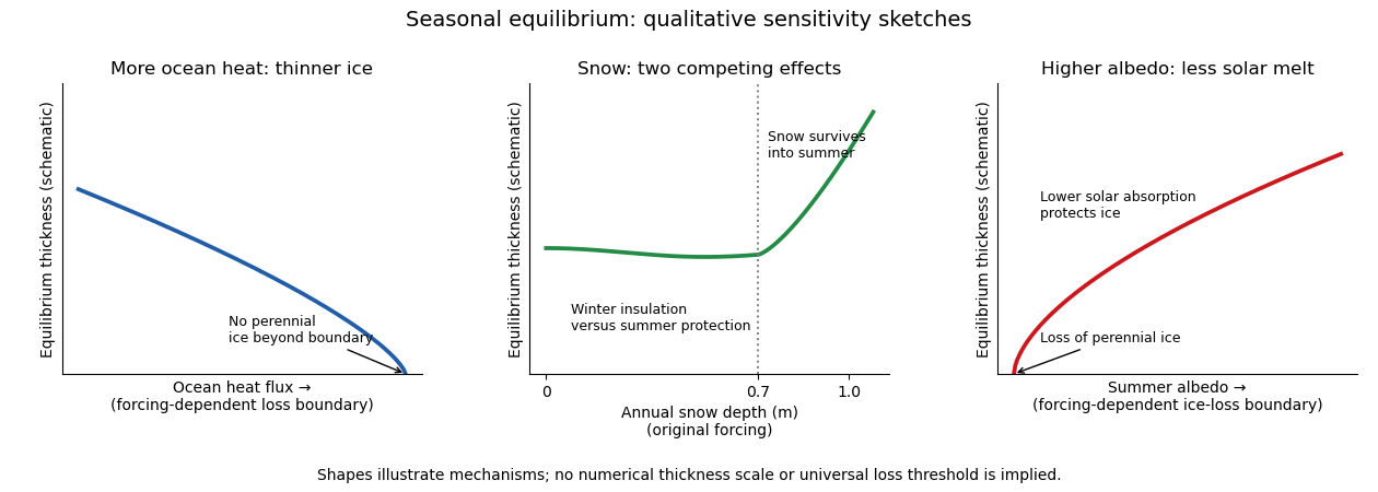
Three schematic equilibrium-thickness sensitivities: ocean heat flux, annual snow depth and summer albedo
. Details. The three curves are original qualitative sketches, not a new numerical integration or digitization. The snow marker refers to that historical forcing; the unnumbered loss boundaries and ordinate indicate trends rather than calibrated universal thresholds.
For the summer retreat discussed around the time of this examination, the proposed mechanisms act as follows.
- Warmer air increases sensible heat input when the air is warmer than the surface, often accompanies increased downward longwave radiation, advances spring melt and delays autumn cooling. Air temperature alone does not determine the surface energy balance: cloud, humidity and circulation changes affect the radiative terms as well. It is a broad climatic forcing, but cannot explain all local basal melt without an ocean energy pathway.
- Extra Atlantic-layer heat is a potential subsurface reservoir. A cold, fresh halocline can isolate it from the surface, so a warmer Atlantic layer does not by itself imply the same heat flux at the ice. Its influence is stronger in regions where warm inflow is shallow or mixed upward, especially toward the Atlantic sector.
- Erosion of the cold halocline removes that insulation. Reduced density stratification or stronger mixing can bring Atlantic heat upward, producing increased ocean heat flux and basal melt. This is an enabling mechanism, not an independent creation of heat to be added twice to the Atlantic contribution. Atlantic-water and stratification measurements support the coupling of these changes.
- Pacific inflow through Bering Strait supplies upper-ocean heat to the Chukchi and western Arctic. It can melt ice locally and precondition the Beaufort region for earlier retreat; its importance is regional and seasonal, rather than uniform over the basin. observations of Pacific summer water and western-Arctic ice retreat support this pathway.
- Changes in the Arctic Oscillation alter winds, ice drift, convergence and export through Fram Strait. Enhanced export can remove old thick ice, expose more open water and change the following year's thickness distribution. An index phase is not a direct heat flux, nor does a single phase explain every summer anomaly. ice-age and drift reconstructions show how circulation can precondition summer loss.
- Long-term thinning reduces the latent heat needed to remove a floe and replaces persistent multi-year sea ice by vulnerable younger ice. It also makes the cover easier to deform and disperse. This accumulated preconditioning amplifies summer forcing, while faster winter growth of thin ice provides a partial negative feedback.
- Lower albedo of melt ponds, bare ice and open water increases solar absorption. Heating of leads and the upper ocean feeds basal and lateral melt, making ice-albedo feedback a strong summer amplifier.
These processes overlap: circulation causes export, export changes thickness and open-water fraction, and those changes alter solar absorption. Without specified regional budgets there is no defensible unique percentage partition. For enhanced Beaufort summer basal melt, upper-ocean solar heating and western-Arctic heat pathways are more directly relevant than invoking unmodified heat from a deep, isolated Atlantic layer. ice-mass-balance observations of extreme Beaufort melt identify increased solar absorption in open water as an important source.
Take as an explicit ice-density approximation and use the supplied . The latent heat for basal ablation isJune–September contains about days, soUsing would give . This is the net flux used for melting: the gross ocean heat flux can also supply conductive losses and changes in cold content. It greatly exceeds an annual central-pack background of a few , but is compatible with a summer upper ocean absorbing solar radiation at tens to hundreds of . For scale, an added open-water fraction , a shortwave input and an ice–water albedo contrast produce additional area-mean absorption before losses. This is an illustrative budget, not a measurement. Wind mixing and circulation can deliver stored solar or advected heat to the underside.
The ice-albedo feedback closes the warming loop: retreat exposes darker water; extra solar absorption warms the upper ocean; basal and lateral melt increase retreat. The stored heat also delays autumn freeze-up, exposing water to atmospheric heat transfer for longer. Its later release warms the atmosphere, but must not be counted as a second source in addition to the solar energy that originally entered the ocean. In winter, greater heat loss from open water and rapid growth of thin ice partly oppose the summer positive feedback.
Let be ice velocity, air velocity and water velocity in an Earth-fixed frame. Put and . For effective air and water drag areas , a quadratic drag convention commonly used for geophysical stresses givesThe Coriolis force magnitude is , while its sign is retained in the vector equation. The coefficients here incorporate any conventional factor ; if one uses , then describes the same resistance. Windage and water drag areas must be declared: an iceberg can have pressure drag on its exposed and submerged faces as well as basal skin drag. They cannot generally be inferred from ice mass alone.
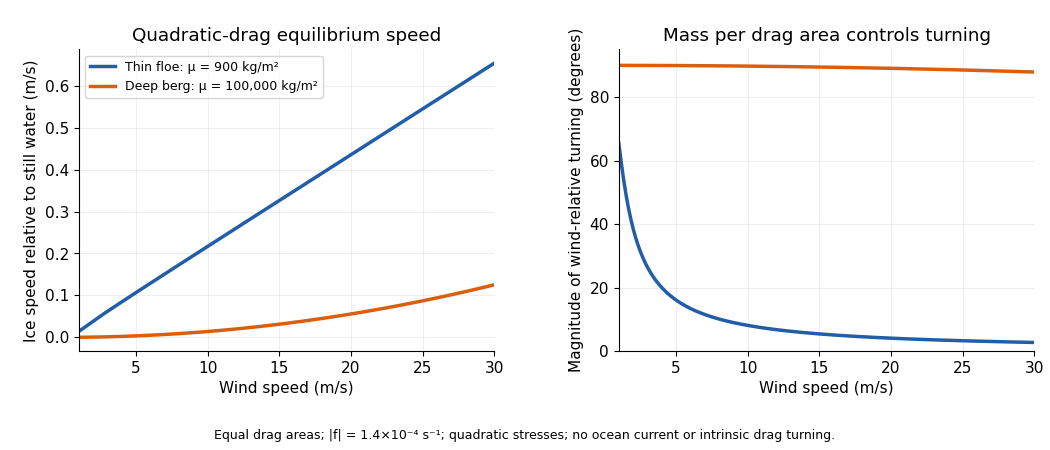
To obtain an explicit quadratic-drag turning angle, first take still water and no sea-surface slope, and suppose . Then the wind force is approximately with , while water resistance remains quadratic. Steady free drift satisfiesIn the northern hemisphere write with . Resolving parallel to the drift and toward its left givesSquaring and adding eliminates , rather than replacing water resistance by a fixed linear coefficient:The positive root and angle are thereforeThe stable root displayed avoids subtracting nearly equal large quantities. The drift is to the right of the wind for and to the left for . Define the mass per drag area , the area ratio , the wind stress scale and the water-drag coefficient . Dividing the force balance by givesIn particular, has units , not metres. A convenient dimensionless form isThe cosine follows by substituting into the along-drift equation, giving . Thus wind speed, drag coefficients and latitude are insufficient without mass and area normalization.
For , water drag dominates the turning correction:For , Coriolis force dominates the cross-wind balance:The cross-wind force does no work. Multiplying the original equilibrium equation by gives , which independently verifies the along-drift relation.
If the small ice-speed approximation is unsuitable, retain relative wind in the original equation. In still water the two exact steady component equations, with and , areConsequently and , together with the definition of . These equations determine the exact angle and speed implicitly and reduce to the explicit formulas above when and . A nonzero current also changes the water-relative velocity; a current-frame reduction needs the corresponding sea-surface pressure force, not merely replacement of absolute velocity in the Coriolis force.
A thin ice floe has small , so appreciable wind produces relatively rapid, nearly downwind motion in this idealized model. A deep iceberg generally has a much larger and often a smaller effective windage-to-water-drag ratio. Its wind-driven motion relative to the ocean is slower and more nearly across the wind; ambient currents can then dominate its absolute trajectory. For example, taking , , , , , and , the formulas give about , for , versus , for . These are examples with the stated areas and coefficients, not universal observed turning angles. Boundary-layer turning, form drag and pack stresses can change them. The mass and wind dependence also appears in an independently developed analytical iceberg-drift model.


In the Antarctic, reverses the wind-relative turning. Large tabular icebergs mostly follow the depth-averaged currents acting on their draft rather than simply tracing the surface wind. The westward coastal circulation can retain or carry them around the continent, whereas offshore access to the eastward circumpolar circulation enables long-range export. Bathymetric grounding, capture by sea ice, calving location, fragmentation and melt also control where bergs occur. As a berg breaks into smaller pieces its mass-to-drag-area and windage ratios change, so the wind response can change before it melts. The derived turning tendency alone cannot predict a distribution map.
Other forces should be compared as forces per horizontal area, using the same normalization. For an illustrative wind and the above air parameters, the wind stress is when the air drag area equals the horizontal area.
- Water currents and tides change quadratic drag. A relative water speed gives , about one fifth of this wind stress; gives , over five times as large. Currents and tides are therefore often leading-order, particularly for deep icebergs.
- A sea-surface slope produces a horizontal pressure gradient force , or stress magnitude . With a representative geostrophic balance, . For , this is for the floe and for the deep berg above. Much of this force balances the Coriolis force associated with following the ocean current; counting it as an independent extra wind driver would double-count that balance.
- Acceleration matters during changes of forcing: its stress scale is . Changing speed by in six hours requires for the floe, but for the deep berg. Thus large bergs adjust slowly and a steady solution need not apply to a short wind event.
- Contact forces and internal pack stress invalidate free drift in compact ice. An illustrative integrated compressive stress changing across gives , larger than the reference wind stress. Floe collisions and grounding can momentarily exceed it by much more; grounded ice can remain stationary regardless of the free-drift angle.
- Waves transfer momentum when absorbed or reflected. For a wave of amplitude , energy per area is about . With deep-water phase speed and group speed , complete absorption across a width gives force per unit width , about . Dividing by an along-wave floe length gives , but this is an absorption bound; transmitting most of the waves reduces it greatly. Reflection, wave spectrum, ice attenuation and geometry must be specified before assigning an actual wave force. The same perimeter force divided by a giant berg's much larger area is relatively smaller.
These estimates declare their scales; there is no single universal ratio for every floe, iceberg and sea state. Direct atmospheric pressure-gradient stress, for comparison, is roughly ice thickness times atmospheric pressure gradient: for a thin floe. Wind stress, currents, ocean pressure gradients, contact forces and waves usually require separate treatment.
For the towing estimate, use the specified basal areaWith the declared stress convention and relative water speed, quadratic drag isThe tug fraction is . In a one-dimensional incremental drag balance, even a favourably aligned pull changes speed only byInterpreting the printed coefficient with an explicit convention instead gives and doubles these tiny fractions, without changing the conclusion. Buoyancy gives ; a high-latitude Coriolis force at is , also far beyond the tug force. With resistance ignored altogether, the tug acceleration is only .
There is a further source qualification. Sustaining this giant berg at relative to still water would require an unusually enormous driving force; ordinary winds with the illustrative coefficients supply only . A measured absolute velocity may primarily follow a current, in which case the drag calculation needs its relative velocity rather than . Under the stipulated relative-motion interpretation, one such tug cannot significantly change the motion, and these numbers provide no support for a long-distance tow of this giant berg. They do not disprove towing every smaller iceberg: feasibility changes with area, draft, relative tow speed, available tug force, currents and melt losses.
A convective chimney is a localized, deeply mixed region within a stratified ocean, formed when surface buoyancy loss allows convection to penetrate far below the surrounding mixed layer. The chimney describes the mixed water column and its circulation; instantaneous downward transfer occurs through many smaller plumes, accompanied by compensating motion and lateral exchange, rather than through one permanently uniform downward pipe. Open-ocean convection occurs in the Labrador and Irminger Seas, the Greenland Sea, the northwestern Mediterranean, and episodically in the open Weddell Sea under a large polynya. Dense-water formation on a continental shelf is related but geometrically distinct from deep open-ocean chimney convection.
Observed Greenland Sea convective chimneys include compact, approximately circular, weakly stratified cores with temperature and salinity much more uniform vertically than in the ambient ocean. A mapped example was about across, extended to about in winter, and rotated anticyclonically. In summer a fresh, low-density cap and shallower lateral intrusions could isolate the deep core, while winter buoyancy loss removed the cap and renewed deep contact. Such cores could persist through several seasons, so presence of a deep homogeneous core is not proof that vigorous convection is occurring continuously. These particular dimensions and seasonal structure come from successive hydrographic surveys of Greenland Sea chimneys.
Formation is favoured by the cyclonic Greenland gyre, which domes density surfaces and can reduce the depth of the stratified barrier. Cold, dry wind outbreaks produce strong sensible, latent and longwave heat loss. Where frazil ice and pancake ice form in the Odden ice tongue, ice growth removes relatively fresh material while brine rejection increases the density of the remaining water. Ice advection can keep exposing water for further freezing and separate local brine release from later freshwater return. This combination of preconditioning, cooling and sustained salt input can make a formerly buoyant surface layer dense enough to convect.
Conversely, a fresh surface cap supplied by Arctic freshwater and ice melt strengthens density stratification. Warmer atmospheric outbreaks reduce surface heat loss and ice production; circulation changes affecting the cold northwesterly winds and the Odden can reduce the brine source. Atlantic advection supplies both heat and salt, with competing effects on density, so temperature alone is not an adequate diagnostic. The historical decline in Odden ice formation and changes in wind regimes offer a mechanism for less favourable chimney production around the period considered, but ice-driven formation is a physical hypothesis, not evidence that every observed chimney requires ice or that every local change follows a single climate index. The Greenland Sea salt-flux model explicitly includes ice production and advection.
For the brine rejection mechanism, let be ice growth and let be water and ice salt mass fractions. Newly formed ice removes mass per area per time. Compared with removing water at concentration , it leaves an excess salt flux in the liquid ofThe units are . With the exam's approximation for salinity in psu, the corresponding mixed-layer salinity tendency is, to first order,If , the surface buoyancy input is negative, with scale . The enhanced density produces downward saline plumes that deepen mixing if this buoyancy loss overcomes the available density stratification. This explains why exporting new ice while retaining its rejected salt can strengthen overturning, whereas later local melt reverses the freshwater effect.
For the numerical comparison, the cover gives the specific heat capacity of ice, not of seawater. A seawater value must therefore be supplied explicitly. Take and use the stipulated . A column has initial water mass per areaCooling it by removesThe specified thermal density relation givesThis assumes the whole column mixes and neglects entrainment and advected heat. Using the supplied ice heat capacity for liquid seawater would change incorrectly.
At the freezing point the same heat extraction produces a pure-ice mass per areaHere is the fraction of the original water mass removed into ice. With the explicit ice-density approximation , the resulting ice thickness isThe water-equivalent thickness uses a reference water density: with fresh water at , it is . The depth of the original seawater removed is instead . These three quantities are different; is not the physical ice thickness for the stated density approximation.
Let the initial salinity be . Complete exclusion of salt from the ice leaves all the initial salt in a liquid mass . Conservation of salt during freezing givesThe initial salinity is not printed, so a unique numerical salinity increase requires another explicit assumption. For ,The total density increase after cooling followed by freezing is then about . The factor is required because salt concentration refers to the remaining liquid mass. Using ice thickness divided by the original water depth as the removed mass fraction would violate this accounting.
For this assumed salinity, the freezing-to-cooling density efficiency shows that equal heat extraction at freezing produces about times the density increase of the initial cooling. At low temperature the thermal expansion response is weak, whereas brine rejection changes salinity efficiently. This supports strong freezing-driven convection where water is already near its freezing point. It does not mean freezing always creates deep chimneys: the initial density stratification, freshwater supply, mixing depth and later melting remain decisive. The freezing point itself decreases as salinity rises; keeping it at is the exam's approximation. Allowing that small additional cooling and a temperature-dependent equation of state would require a refined heat budget.
Important other sites of freezing-enhanced downward transfer include the Ross and Weddell Antarctic shelves and their coastal polynyas, Adélie Land and Cape Darnley, Arctic shelves such as the Barents and Kara Seas, and the Sea of Okhotsk. On shelves the saline dense water can cascade down a continental slope and feed deeper waters; the same salt-removal balance operates without requiring an isolated open-ocean chimney. A later direct observational example is bottom-water formation associated with Cape Darnley sea-ice production.
Atmospheric warming of the Greenland Sea can reduce surface cooling and ice formation, while increased freshwater input can inhibit convection. If these changes weaken the Atlantic meridional overturning circulation and its northward heat transport, their ocean-mediated tendency is relative cooling, or reduced warming, of northwestern Europe compared with otherwise identical atmospheric warming. This is not a prediction of net European cooling under all emissions scenarios, nor does one chimney determine the whole overturning circulation: other convection regions, winds, freshwater pathways and coupled ocean adjustment also matter. The physical conclusion is the sign of the heat-transport response, not a specified century-scale temperature decrement.
Articles by others on the same topic
There are currently no matching articles.