Past exam of the mathematics course of the University of Cambridge / 2014 / iii / Paper 42 / 1

An order parameter distinguishes thermodynamic phases and transforms under the symmetry that may be broken. For a scalar ferromagnet it is the magnetization per site; a disordered zero-field phase has $m=0$, while ordered pure thermodynamic phases have $m=\pm m_0$. In a fluid one can instead use the density measured relative to its critical value; the field conjugate to it is then related to the chemical potential rather than literally a magnetic field. A nonzero value in the presence of an explicit conjugate field is not by itself evidence of a spontaneous transition.

The LG theory describes a slowly varying local order parameter by a symmetry-constrained free-energy functional, for exampleAt $h=0$, a ${\mathbb{Z}}_2$ symmetry excludes odd powers. The coefficients are assumed analytic functions of the controls near the transition, and the expansion is stabilized by a positive highest retained even coefficient. The Landau approximation obtains equilibrium by minimizing this functional, neglecting long-wavelength fluctuation corrections. Its nonconvex local potential describes distinct candidate phases and mean-field metastability; the exact thermodynamic potential is convexified when macroscopic mixtures are admitted.

In a finite symmetric system, the zero-field expectation of $m$ can vanish even below the transition because both ordered orientations are sampled. Spontaneous order is defined by taking the thermodynamic limit before removing a selecting field, for example $m_0={\lim }_{h\downarrow 0}{\lim }_{N\to \infty }⟨m⟩$. This distinction also matters for the connected correlations used below.

A first-order phase transition has a discontinuity in a first derivative of the equilibrium free energy, such as the entropy or order parameter. It can have latent heat when the entropy jumps. A continuous phase transition has a continuously vanishing order parameter and no latent heat, with singular higher derivatives and a diverging correlation length. The LG theory compares global minima, not merely the points where a local minimum loses stability.

For the uniform quartic Landau free energythe equation of state is $rm+u{m}^3=h$. At zero field the stable minimum is $m=0$ for $r>0$, and $m=\pm \sqrt{-r/u}$ for $r<0$. Thus tuning $r$ through zero gives a continuous transition. For a fixed $r<0$, varying $h$ through zero instead switches between the two ordered minima and makes $m$ jump, giving a first-order phase transition in the conjugate field.

A temperature-like first-order transition can occur at zero field when $u<0$ and a positive sextic term $v{m}^6/6$ stabilizes the potential. Write $q=m^2$. Stationarity of a nonzero phase gives $r+uq+v{q}^2=0$, while equality with $V(0)=0$ gives $rq/2+u{q}^2/4+v{q}^3/6=0$. Solving these two conditions yieldsThe order parameter jumps from zero to $\pm \sqrt{q_{\mathrm{coex}}}$. At this pointso the competing stationary points are genuinely global minima. This phase coexistence condition differs from the spinodal points $r=0$ and $r=u^2/(4v)$, which mark loss or creation of local stability, not equilibrium coexistence.

If the symmetry permits a cubic term $w{m}^3/3$, a positive quartic coefficient does not preclude a first-order transition. For $V=r{m}^2/2+w{m}^3/3+u{m}^4/4$ with $w\ne 0,u>0$, stationarity and coexistence give $m=-2w/(3u)$ and $r=2w^2/(9u)$. This is the first-order transition in a cubic-quartic Landau potential; the symmetry restriction on the expansion is therefore part of the prediction.

Along an isolated two-phase coexistence line, two distinct stable minima have equal free energy. If this line ends at an ordinary interior endpoint without encountering another phase, the distinction between the two phases must disappear: their minima and the intervening barrier merge. For separated nondegenerate minima, their stationary values are smooth functions of the controls. The difference $\Delta V=V(m_1)-V(m_2)$ has ${\partial }_h\Delta V=-m_1+m_2\ne 0$. The implicit function theorem therefore continues the equation $\Delta V=0$ as a local coexistence curve. It cannot end while those distinct stable minima persist.

At the merger the potential satisfiesThe third-derivative condition is essential: a stationary zero-curvature point with nonzero third derivative is an inflection, not a stable equilibrium. Shifting to $\psi =m-m_c$ gives an ordinary quartic Landau free energy with two independent control directions, temperature-like and field-like. The curvature and the order-parameter discontinuity vanish, the magnetic susceptibility diverges, and the correlation length diverges. The endpoint is therefore associated with a continuous transition. This is the critical endpoint of a quartic Landau free energy mechanism.

In the symmetric quartic example, the coexistence line is $h=0,r<0$. Its jump $2\sqrt{-r/u}$ vanishes at $(r,h)=(0,0)$, where $V=u{m}^4/4$. This supplies a concrete realization. The word “must” requires the stated ordinary-endpoint assumptions: a first-order line can instead meet a third phase, a multicritical point, a boundary of parameter space, or continue without a finite endpoint. A spinodal point alone is not an equilibrium critical endpoint.

Critical exponents describe leading power-law singularities as the reduced temperature $t=(T-T_c)/T_c$ and the conjugate field tend to zero. Their amplitudes depend on microscopic details, while the exponents are characteristic of a universality class. Define $m_0\sim (-t{)}^{\beta }$ on a selected ordered branch, $\chi \sim |t{|}^{-\gamma }$ at zero field, $C_{V,s}\sim |t{|}^{-\alpha }$ for the singular heat capacity, and $m(t=0,h)\sim \mathrm{sgn}(h)|h{|}^{1/\delta }$. Also define $\xi \sim |t{|}^{-\nu }$ and $G(r,t=0)\sim r^{-(D-2+\eta )}$. In these statements $\beta$ is the order-parameter critical exponent, not inverse temperature.

Assume $r=r_{t}t$ with $r_t>0$ and a nonzero positive quartic coefficient $u$. Minimizing the quartic potential gives $m_0=\sqrt{-r/u}$, hence $\beta =1/2$. Differentiating its equation of state givesso $\gamma =1$ with different amplitudes. At $r=0$, $h=u{m}^3$, giving $\delta =3$. The minimized potential is zero above the transition and $-r^2/(4u)$ below, so its second temperature derivative has a finite jump: $\alpha =0$.

The quadratic fluctuation kernel around the stable uniform minimum is $\kappa p^2+V^{\prime \prime }(m_0)$, so ${\xi }^2=\kappa /V^{\prime \prime }(m_0)$. Since $V^{\prime \prime }$ is $r$ above and $-2r$ below, $\nu =1/2$. Its critical momentum dependence is $p^{-2}$, giving $\eta =0$. Thus the ordinary mean-field critical exponents areThese are predictions of the Landau approximation, whose validity is constrained by the Ginzburg criterion; they need not be the exponents of the fluctuating theory below its upper critical dimension.

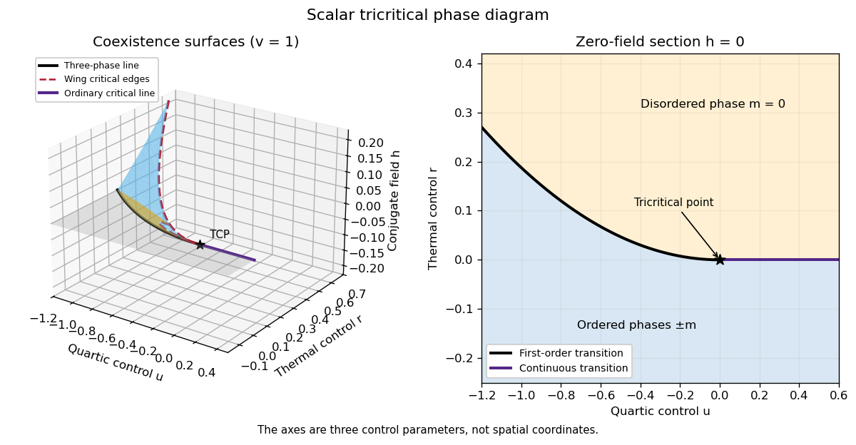
A tricritical point joins continuous and first-order transition loci and requires tuning an additional temperature-independent control. In the scalar sextic potentialit occurs at $r=u=h=0$: both the quadratic and quartic terms vanish. At $h=0,u>0$, the transition is continuous at $r=0$; at $h=0,u<0$, it is first-order at $r=3u^2/(16v)$. The jump tends to zero as $u\uparrow 0$, so these loci meet at the tricritical point.

For the three-control phase diagram with coordinates $(u,r,h)$, the sheet $h=0$ below these transition loci has coexistence of the two ordered phases. For $u>0$ its boundary is the ordinary continuous critical line $r=h=0$. For $u<0$ the boundary $r=3u^2/(16v),h=0$ is a tricritical three-phase line, where $m=0$ and $m=\pm \sqrt{-3u/(4v)}$ all coexist. Two symmetry-related tricritical wings extend from that line into $h>0$ and $h<0$, describing first-order coexistence between small- and large-magnitude phases of the same sign. Each wing ends along an ordinary wing critical edge.

The critical-edge conditions $V^{\prime }=V^{\prime \prime }=V^{(3)}=0$ giveHere $V^{(4)}(m_c)=-12u>0$, so these are ordinary quartic endpoints. The two wing critical edges and the zero-field ordinary critical line are three continuous critical lines meeting at the tricritical point; the three-phase first-order line also ends there. The “3D” phase diagram refers to three independent controls; it is distinct from the spatial dimension $D$ of the field theory.

The figure uses actual sextic-potential coexistence surfaces rather than drawing arbitrary wings. For two coexisting nonnegative minima $a\le b$, put $s=a+b,q=ab$. The tricritical wing coexistence factorizationholds when $u=(2v/3)(-2s^2+3q)$, $r=(v/3)(s^4-s^{2}q+3q^2)$ and $h=(v/3)s^{3}q$. It proves that both minima are globally stable. The limits $q=0$ and $q=s^2/4$ produce the three-phase line and critical edge, respectively; reflection gives the other wing.

At $u=h=0$, $m_0=(-r/v{)}^{1/4}$ on the ordered side and $V(m_0)=-(-r{)}^{3/2}/(3\sqrt{v})$. At the critical isotherm $h=v{m}^5$. Thus the tricritical mean-field critical exponents areThe source's extra control is required to tune $u$ to zero; simply changing temperature in a generic quartic system does not produce tricriticality. The tricritical upper critical dimension is three, as established in Question 3.

The scaling hypothesis for critical phenomena says that the singular part of the equilibrium free energy is a generalized homogeneous function of its thermal and field-like controls. Smooth backgrounds must first be removed; the hypothesis does not claim that the entire free energy, including arbitrary regular terms, has a pure scaling form.

For the ordinary scalar quartic LG theory, set $r=r_{t}t$ with $r_t>0$ and $u>0$, and rescale the uniform order parameter asThe order-parameter-dependent free-energy density becomesDefine $f_{\pm }(H)$ as the minimum of the braces, with the sign of the quadratic term respectively positive or negative. ConsequentlyFor an extensive $A_s$, $a$ additionally contains the system volume. The printed double-inequality subscript labels the two temperature branches: the upper-temperature function is $f_{+}$ and the lower-temperature function is $f_{-}$. It does not classify positive and negative magnetic fields. In particular $f_{+}(0)=0$ and $f_{-}(0)=-1/4$; below the transition the field dependence has a cusp at zero, so derivatives are taken on a selected branch.

For the following derivatives, take $A_s$ to be a density, so $m$ is the magnetization density; for total free energy the derivative gives total magnetization instead. Differentiate this mean-field scalar free-energy scaling form. The magnetization is $m=-\partial A_s/\partial h=-ab|t{|}^{1/2}{f}_{\pm }^{\prime }(H)$, giving $m_0\propto (-t{)}^{1/2}$ and $\beta =1/2$. The magnetic susceptibility is $\chi =-{\partial }_h^2{A}_s=-a{b}^2|t{|}^{-1}{f}_{\pm }^{\prime \prime }(H)$, giving $\gamma =1$. At zero field the nonzero curvature amplitudes are $-f_{+}^{\prime \prime }(0)=1$ and $-f_{-}^{\prime \prime }(0^{+})=1/2$.

To allow nonclassical critical exponents, replace the fixed powers byThe heat-capacity critical exponent is defined by $C_{V,s}\sim |t{|}^{-\alpha }$; temperature differentiation gives the thermal exponent $2-\alpha$ in $A_s$. The order-parameter critical exponent has $m_0\sim (-t{)}^{\beta }$, and the magnetic-susceptibility critical exponent has $\chi \sim |t{|}^{-\gamma }$. Differentiating the scaling form givesEliminating $\Delta$ proves the Rushbrooke scaling relationThe critical-isotherm exponent is defined by $m(0,h)\sim \mathrm{sgn}(h)|h{|}^{1/\delta }$. At fixed small $h$, the $t\to 0$ limit requires $f_{\pm }(H)\sim c|H{|}^{(2-\alpha )/\Delta }$, so that the temperature factors cancel. Therefore $1/\delta =(2-\alpha -\Delta )/\Delta =\beta /\Delta$, yielding $\Delta =\beta \delta$. But the two differentiated identities also give $\Delta =\beta +\gamma$, and hence the Widom scaling relationThese are relations among the leading power indices. At marginal dimensions, multiplicative logarithms can accompany them, and an additive analytic background must not be mistaken for the singular scaling contribution.