Use geometrized units and metric signature , with . In the exterior of Schwarzschild spacetime, put . The Schwarzschild tortoise coordinate satisfiesThe retarded and advanced null coordinates and then give . The logarithmic divergence of suggests exponentiating these null coordinates. In the right exterior define the Kruskal–Szekeres coordinatesTheir product eliminates :Since and , the Schwarzschild metric becomesHere is an implicitly defined function of . The derivative of the right side with respect to is , which is nonzero at . The inverse function theorem therefore makes smooth across that surface, and the coefficient of tends to . Thus the Schwarzschild event horizon is a coordinate singularity of the original chart, while this Lorentzian metric remains regular there.
Extend the Kruskal–Szekeres coordinates to all real with . The signs give two exterior regions, and , a future black hole region , and a past white hole region . The event horizons are or , intersecting at the bifurcation surface. The boundary has and is a genuine Schwarzschild singularity, as the Kretschmann scalar diverges there.
Finally, and give and a radial metric proportional to . Hence radial null geodesics have slopes , the event horizons are , and the singular boundaries are . This constructs the maximal Kruskal extension; a black hole produced by collapse need not contain the second exterior or the white hole of that eternal extension.
Start with the four-dimensional Minkowski metric , where . Choose an arbitrary length , and use the retarded and advanced null coordinates , . For the Minkowski conformal compactification, setBoth lie between and . Since , we have ; the remaining inequalities are . Moreover,Multiply by the square of the conformal factor . The resulting metric is regular on the appropriate boundary pieces and preserves the null directions. Suppressing the angular two-spheres gives a triangular Penrose diagram with radial null geodesics at degrees.
The line is the ordinary timelike centre . The upper sloping edge is future null infinity, reached with and finite ; the lower sloping edge is past null infinity, reached with and finite . The vertices and are future and past timelike infinity, denoted and . The vertex is spacelike infinity, . These are limiting endpoints in the conformal completion, rather than ordinary physical events. In particular, finite diagram coordinates at null infinity do not imply finite physical affine parameter.
The four-dimensional radial diagram is the triangle , . If one instead draws two-dimensional Minkowski spacetime with a signed Cartesian spatial coordinate, the diagram is the full diamond. The centre is a boundary of the radial quotient, not a boundary of the physical four-dimensional Minkowski spacetime.
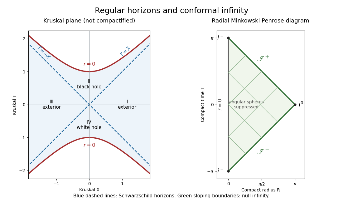
Kruskal extension and the radial Minkowski Penrose diagram
. Details. 
The physical argument for the Penrose inequality combines weak cosmic censorship conjecture, the dominant energy condition, and relaxation to a stationary black hole. Work in geometrized units. Let and be the final Kerr black hole mass and horizon area. Positive energy radiated to infinity gives , where is the initial ADM energy. For a Kerr black hole with ,If the initial apparent horizon obeys the necessary apparent-horizon area comparison with the enclosing event horizon, and Hawking's area theorem applies during the evolution, thenConsequently the anticipated answer, under those additional hypotheses, isThe bound is saturated by a nonrotating Schwarzschild black hole with no energy loss. Rotation or outgoing radiation makes the argument's inequalities stricter.
There is an essential qualification: inclusion inside an event horizon does not by itself compare areas. An arbitrary apparent horizon on general, non-time-symmetric initial data need not satisfy the displayed apparent-horizon area comparison; the unqualified version with its area is not universally true, even with the dominant energy condition. On time-symmetric data the relevant outermost minimal surface is an outer area-minimizing surface, as used in the Riemannian Penrose inequality, with nonnegative scalar curvature. In more general formulations an appropriate enclosing-area quantity is needed. The physical expectation is conditional on this area comparison, as well as on censorship, predictability, settling, and the energy assumptions; the mere presence of a trapped surface does not supply every step.
A null geodesic congruence is a smooth local family of null geodesics, with one generator through each point of the region being described. Choose an affine parameter on each generator and write . Before a caustic, is a smooth, nonzero null vector field satisfying and .
With , compatibility of the Levi-Civita connection with the metric givesThe geodesic equation with affine parameter gives the other contraction:Thus both contractions vanish. Nullness supplies the first identity, and affine parametrization supplies the second; a general nonaffine tangent would instead have .
Choose a local transverse three-dimensional section of the null geodesic congruence and a future unit timelike vector on it. Orient to the future and put . On that section define a parallel auxiliary null vector by the initial valueSince , , and , direct contraction gives and .
Extend along each generator by parallel transport, solving with those initial values. The geodesic equation and compatibility of the Levi-Civita connection implyTherefore , , and hold throughout the local congruence. Smooth initial data and the transport equation give a smooth field up to the breakdown of the congruence at caustics. An arbitrary pointwise choice of away from the initial section would not automatically have this transport property.
The screen-space projector annihilates both null vectors: , and satisfies . Its image is the two-dimensional spacelike screen orthogonal to . The screen metric isIt is positive definite on that screen. Projecting both indices of gives the optical tensor .
Define its three parts byThus . The null expansion is its trace and equals for the infinitesimal beam area . The null shear is symmetric and trace-free, measuring shape change at fixed first-order area. The null twist , also called rotation, is antisymmetric and measures failure of screen directions to remain hypersurface-orthogonal. In dimensions replace by . Here and below expansion means the trace, rather than its average over the screen dimensions.
Locally write the null hypersurface as . Its generators are tangent to its raised normal, so on it for a nonzero scalar . The antisymmetric derivative issince the Hessian of is symmetric for the torsion-free Levi-Civita connection. Each term contains , which is proportional to and is killed by the screen-space projector. HenceThis is the null version of hypersurface orthogonality in the Frobenius theorem. A null hypersurface has no independent normal direction outside its tangent space: its null vector normal also generates it. That is why the same argument applies to the generators' null twist.
For the round sphere, every normal has only components because the Reissner-Nordstrom metric has no mixed angular terms. The vector is normal and null: . Write the second null vector normal as . The normalization gives , so . Its null condition then reads . ThusThe specified future orientation of , together with , makes future-directed as well. This choice fixes the reciprocal scaling freedom of the two null vectors on the sphere.
For each of the two normal directions, launch a null geodesic congruence orthogonally from the sphere with initial tangent or . For take initial auxiliary ; for take initial , and then parallel transport as in part (a). On the sphere the resulting screen-space projector projects onto its angular tangent space, whose metric is .
For any radial normal , the spherical null expansion in ingoing coordinates follows directly from area variation:Equivalently gives . ConsequentlySpherical symmetry also makes the null shear and null twist zero for these radial congruences.
There is a small parametrization distinction. The smooth field is affine, since . The natural smooth field obeys . To meet part (a)'s affine convention, use an affine rescaling of a null normal along the outgoing generators, with scaling equal to one on . Its angular derivatives on then leave the projected derivative unchanged. The displayed null expansions are therefore precisely those for the affinely launched congruences, even though that convenient global expression for is nonaffine away from its initial sphere.
A future trapped surface is a closed spacelike two-surface for which both future orthogonal null expansions are strictly negative. Multiplying a future null vector normal by a positive function multiplies its null expansion by that function, so the signs are invariant under allowed normalization changes.
Here for every . Thus the Reissner-Nordstrom trapped spheres are exactly those with . Since ,At either horizon , so the spheres are marginal, rather than strictly trapped surfaces. For or , and this future-trapping condition fails. In particular, being inside the outer event horizon alone is insufficient to make every sphere trapped in the charged solution.
One standard form of the Penrose singularity theorem assumes a time-oriented globally hyperbolic spacetime with a noncompact Cauchy hypersurface, the null convergence condition for every null vector , and a closed future trapped surface. It concludes future null geodesic incompleteness: some future-inextendible null geodesic has a finite upper endpoint of its affine parameter.
The focusing mechanism is the Null Raychaudhuri equation. The normal generators have zero null twist, soAn initial therefore gives a conjugate point to a spacelike surface within affine distance at most , assuming the generator can be continued that far. Such a generator ceases to lie on the achronal boundary after its first focal point. Compactness of the trapped surface supplies a uniform bound for all normalized initial null normals. Future completeness would consequently make its future boundary compact. Projection along timelike curves to a connected Cauchy hypersurface is injective on the achronal boundary and has open image. Compactness makes the image closed as well; the nonempty image must therefore be the entire hypersurface, contradicting its noncompactness. This explains why the global assumptions supplement local focusing.
For Reissner-Nordstrom spacetime, the Maxwell stress-energy tensor satisfies the null energy condition; the Einstein field equations imply the required null convergence condition. The spheres in the band just found are closed and trapped. Apply the theorem to a maximal Cauchy development with a noncompact Cauchy hypersurface and containing one such sphere. That globally hyperbolic spacetime must be future null-geodesically incomplete.
The Penrose theorem at a Cauchy horizon needs care: the full maximal analytic Reissner-Nordstrom spacetime has inner Cauchy horizons and is not globally hyperbolic. It does not satisfy every hypothesis of the displayed theorem. In the exact solution some incomplete geodesics of the globally hyperbolic development reach a smoothly extendible Cauchy horizon in finite affine parameter. The theorem asserts incompleteness of the development, not that every such endpoint is a curvature singularity. The separate curvature singularity at does not justify silently dropping the theorem's global hypothesis.
An isolated uncharged collapsing star initially has higher multipole moments and possibly time-dependent motion. The changing exterior emits gravitational waves, carrying away energy and nonspherical structure. Perturbations of the final black hole decay, so the late exterior is expected to approach a stationary spacetime.
Under the regularity, asymptotic flatness, and connected-horizon hypotheses of the black-hole uniqueness theorem, a stationary four-dimensional vacuum black hole is a Kerr black hole. Since the electric charge is zero, its intrinsic parameters areThe black-hole no-hair theorem expresses the loss of independently specifiable higher multipoles: those of the final Kerr black hole are determined by . The direction of the rotation axis can be chosen by orienting the coordinates and is not an additional intrinsic parameter of the geometry.
This is a statement about the settled, isolated exterior in classical general relativity, conditional on settling and the hypotheses of the black-hole uniqueness theorem. It does not describe the entire radiating collapse spacetime with only two numbers, nor does it extend unchanged to additional long-range matter fields.
Write , , , and . Use ingoing Kerr coordinates, so and . To see the cancellations without expanding every term, write the Kerr metric in the equivalent formThe combinations becomeThe first square contributes , cancelling the explicit radial term. Expanding the remaining terms givesThere is no denominator in this Lorentzian metric. At the outer horizon , and the components are smooth. The determinant is , so away from the usual polar-coordinate degeneracy the metric is nondegenerate and extends across . The axis can be covered by regular angular charts. Thus the Boyer-Lindquist coordinates are singular there, while the ingoing Kerr coordinates are regular at the future horizon.
For physical nonextremality the invariant parameter condition is , . The printed is sufficient when the rotation orientation has been chosen so that ; without that convention it needs the absolute value.
The change to ingoing Kerr coordinates adds functions of to and , and leaves unchanged. Differentiating at fixed therefore gives and . Differentiating at fixed gives and . Hence the two Killing vector fields areThey remain the stationary and axial Killing vector fields; the coordinate change does not mix their generators with .
The inverse Kerr metric in ingoing Kerr coordinates gives the raised normal to a surface of constant :On , , so the normal is null and tangent to the horizon. It reduces toA constant linear combination of the two Killing vector fields is again a Killing vector field. Therefore is normal to this null hypersurface, establishing that it is a Killing horizon, with Kerr horizon angular velocityThe second equality uses . This normal calculation proves hypersurface orthogonality on the horizon, rather than merely proving that the proposed vector happens to have zero norm there.
A generator of the Killing horizon is an orbit of . In ingoing Kerr coordinates it has constant and , with . Since the coordinate shifts depend only on , this is also in the limiting Boyer-Lindquist coordinates description.
Thus is the angular velocity of the horizon relative to the nonrotating stationary frame at infinity. The stationary Killing vector field is normalized to unit time translation there, while the axial Killing vector field has -periodic orbits. This normalization makes the Kerr horizon angular velocity physically definite. It describes the rotation of the null generators and the dragging of inertial frames, not a material solid surface rotating through space. In the Schwarzschild black hole limit , .
For the scalar wave separation in Kerr spacetime, continue to use and . First verify the determinant in the hint. Direct multiplication of the covariant components givesHence the block determinant is . Inverting this block givesThe other inverse components are , , and . The covariant wave operator on a scalar consequently has the divergence formLet denote the azimuthal mode number, to distinguish it from the axial vector . Insert the mode in the massless Klein-Gordon equation. Single-valuedness makes an integer. The derivatives giveWith , division by the mode factor gives, on patches where ,The radial and angular expressions must be opposite constants. Defining the separation constant as , we obtain the two ordinary differential equationsThese equations also hold at zeros of a mode by continuity, without dividing there. Regular angular solutions are scalar spheroidal harmonics, with discrete . For the angular equation becomes the associated Legendre function equation, with and , providing a useful check of the signs and normalization. The radial function here is exactly in the chosen ansatz, without an additional factor of .
Fix a classical globally hyperbolic spacetime with metric signature ; in this solution take . A free real Klein-Gordon field can be specified bywhere is its mass, its curvature coupling and the scalar curvature. Global hyperbolicity ensures a well-posed initial-value problem on a Cauchy hypersurface and the existence of retarded and advanced propagators. Thus compactly supported field and normal-derivative data determine a classical solution. This fixes the dynamics, but not a Fock vacuum.
For real solutions with suitable support or falloff, the symplectic form on scalar-field solutions iswith the future unit normal. The field equation makes the current conserved, so this symplectic form is independent of when boundary flux vanishes. Quantize the initial data by the canonical commutation relation: with and the delta function defined relative to , and the two equal-field commutators vanish. Equivalently, construct the field algebra using the causal propagator. A state on that algebra is additional input.
To construct a particle representation, complexify the classical solution space. Its conserved Klein-Gordon inner product isIt is indefinite on all complex solutions. Choose a complete positive-norm subspace and an orthonormal mode basis with , and . Such a choice is encoded by a compatible complex structure on the Klein-Gordon solution space. Its positive subspace gives the one-particle Hilbert space, and the associated bosonic Fock space contains symmetrized many-particle states. The field expansion isThe creation operator adds a particle in mode , the annihilation operator removes one, and the number operator is . For continuous mode labels the sums and Kronecker deltas become integrals and delta functions, or one can work with normalized wave packets.
The ambiguity is precisely that the field equation and global hyperbolicity do not select that positive subspace. A different normalized basis may mix and by a Bogoliubov transformation, and then its annihilation operators mix and . Its Fock vacuum and number operators differ. The Hadamard condition constrains physically acceptable short-distance singularities and allows local renormalization, but it still leaves many states. Hence there is generally no observer-independent particle count on an arbitrary dynamical geometry.
In a stable strictly stationary spacetime, a globally future timelike Killing vector field gives a preferred time translation. Fix its normalization and suitable boundary conditions, and choose positive-frequency solutions satisfying with . The corresponding positive spectral subspace gives the preferred vacuum state in a stationary spacetime. Unitary changes of basis within it leave the vacuum and the particle notion unchanged. This construction assumes a well-defined positive stationary generator; stationarity by itself is insufficient if becomes spacelike, as in a Kerr ergoregion, or if unstable or zero modes obstruct the ground-state construction. It selects a preferred ground state under the stated assumptions, not a unique state among all thermal and excited states.
If the geometry is suitably stationary in the asymptotic past and future, choose those preferred mode spaces separately, giving the in-vacuum and out-vacuum. Propagate the past modes through the intervening region using the field equation and compare them to the future modes using the conserved Klein-Gordon inner product. Adopt the conventionThe canonical identities for a bosonic Bogoliubov transformation read and . Extracting the future annihilation operator with the same inner product givesIn the in-vacuum, only contributes to . Therefore the particle number from Bogoliubov coefficients isNonzero is the production of future particles from the past vacuum. Summing over future modes gives the total expected particle number when that sum is finite. For infinitely many modes, a Hilbert-Schmidt operator is the condition for unitary implementability between these pure bosonic Fock space representations; finite-volume or wave-packet calculations must respect the relevant measures and convergence. Particle production is determined by the negative-frequency mixing, rather than by identifying a single instantaneous vacuum throughout the time-dependent region.
The laws of black-hole mechanics initially relate geometric quantities in a way resembling thermodynamics. Hawking radiation supplies a physical temperature: in units , while displaying ,The Hawking temperature is measured with the stationary time normalized at infinity. The radiation's thermal occupation factor is physically observable; propagation to infinity also introduces greybody factors, so the distant spectrum need not be a perfect blackbody spectrum at every frequency.
The Zeroth law of black-hole mechanics says that surface gravity is constant on a stationary Killing horizon under its standard hypotheses. Through the Hawking temperature, this becomes uniform equilibrium temperature. The First law of black-hole mechanics isUsing identifies its area term as . Integrating gives the Bekenstein-Hawking entropy, up to an additive constant. Thus is the energy, the angular and charge terms are work terms, and the geometrical law is the ordinary thermodynamic first law with a fixed entropy normalization.
The second law of black-hole mechanics, or Hawking's area theorem, gives nondecreasing area in the classical setting with the requisite energy and predictability assumptions. It corresponds to increasing Bekenstein-Hawking entropy. Semiclassical black-hole evaporation can decrease the area: the classical null energy condition need not hold for the quantum expectation of the stress-energy tensor. The appropriate extension is the generalized second law, that does not decrease, with the exterior entropy and its renormalization treated consistently. Hawking's temperature identification motivates this law; thermality alone does not prove every form of it.
The third law of black-hole mechanics is the unattainability, by an admissible finite physical process, of zero surface gravity. With Hawking temperature it becomes unattainability of absolute zero. It is not the assertion that an extremal black hole has vanishing entropy: its area can remain nonzero when .
For a Schwarzschild black hole, and , giving and . Their product satisfies , explicitly checking the first law. Quantum radiation turns the temperature and entropy in the mechanical analogy into physical thermodynamic quantities.
Articles by others on the same topic
There are currently no matching articles.