Past exam of the mathematics course of the University of Cambridge / 2015 / iii / Paper 38 (Mathematics of Operational Research)

For a maximization problem with $g_i(u)\le 0$ and $h_j(u)=0$, use the optimization LagrangianThe Lagrangian sufficiency theorem says: if $u^{\ast }$ is feasible, $u^{\ast }$ globally maximizes $L(\cdot ,{\lambda }^{\ast },{\mu }^{\ast })$ over its original domain, and complementary slackness holds, ${\lambda }_i^{\ast }{g}_i(u^{\ast })=0$, then $u^{\ast }$ globally maximizes $f$ over the feasible set. Equality Lagrange multipliers have no sign restriction. For every feasible $u$,which proves the theorem.

For a minimization problem, reverse the signs in the optimization Lagrangian: take $L=f+{\sum }_i{\lambda }_i{g}_i+{\sum }_j{\mu }_j{h}_j$, with ${\lambda }_i\ge 0$. If a feasible $u^{\ast }$ globally minimizes this optimization Lagrangian and satisfies complementary slackness, thenThe hypothesis is a global extremum of the Lagrangian. Merely solving its stationarity equations is insufficient; no convexity assumption is needed when the global extremum itself has been proved.

With $g=2x-y-z-2$ and $h=x^2+y^2-5$, the maximization optimization Lagrangian isA finite unconstrained maximum requires $\lambda =1$ to cancel the coefficient of $z$. With $\mu =1$, completing the square givesThus its global maximizers have $x=-1$ and $y=2$. The equality constraint holds, and complementary slackness with $\lambda =1$ makes $g=0$, giving $z=-6$. The Lagrangian sufficiency theorem certifiesEvery feasible point has objective at most $L\le 12$, so this is a global conclusion rather than just a stationary-point calculation.

For minimization, the optimization Lagrangian isIts coefficient of $z$ is $-1-\lambda <0$, so its infimum over unrestricted $z$ is $-\infty$ for every allowable Lagrange multiplier. There is no finite global minimizer of the optimization Lagrangian to which the Lagrangian sufficiency theorem could apply.

The primal minimization problem is also unbounded: set $x=0$, $y=\sqrt{5}$ and $z=t\ge 0$. These points are feasible, and $3y-z=3\sqrt{5}-t\to -\infty$. Hence

For any feasible $x,y$, increasing $z$ lowers the objective, so the additional upper bound makes $z^{\ast }=0$. Feasibility then requires $2x-y\le 2$. The lowest feasible value of $y$ on the circle occurs at the lower intersection with $2x-y=2$. Solving gives the candidateA global certificate avoids relying on the circle sketch. Introduce Lagrange multipliers for $g\le 0$, $z\le 0$ and $h=0$:ChooseThe coefficient of $z$ vanishes, and $2\mu x^{\ast }+2\lambda =0$, $2\mu y^{\ast }+3-\lambda =0$. Therefore completing the square yieldsThe candidate minimizes $L$ globally and satisfies both active inequality constraints, so complementary slackness and the Lagrangian sufficiency theorem give

Setting the third coordinate to zero and the first to four leaves $6x_2\ge 4$ and $4x_2\le 3$. Thus $x_2=2/3$ works. Direct substitution givesHence this point lies in both linear polyhedra.

If a vector $h$ gives the strict separation, a common point would satisfy $h^{T}x<h^{T}x$, which is impossible.

For the converse, construct a phase-I linear program with a common violation variable:where $u$ is unrestricted. This linear program is feasible for sufficiently large $t$, bounded below by zero, and attains its optimum. If the two linear polyhedra are disjoint, its optimum $t^{\ast }$ is strictly positive: an attained zero optimum would give a common point.

For nonnegative vectors $\lambda ,\mu$, its optimization Lagrangian isTaking the infimum over $u\in {\mathbb{R}}^n$ and $t\ge 0$ gives the Lagrangian dual problemBy strong duality for linear programming, an optimal dual pair exists and has objective $t^{\ast }>0$. It supplies the infeasibility certificateTake $h=A^T\lambda =-C^T\mu$. Every $x\in P$ and $y\in Q$ obeysThe assumed nonemptiness of each linear polyhedron also ensures $h\ne 0$: if $h=0$, their feasibility would force both ${\lambda }^{T}b$ and ${\mu }^{T}d$ to be nonnegative. This proves the strict separation of disjoint linear polyhedra using Lagrangian duality.

Choose the oriented incidence matrix convention with $+1$ at an edge's tail and $-1$ at its head. Let $b_i$ be net supply, so ${\sum }_i{b}_i=0$. The uncapacitated minimum-cost flow problem on a finite directed graph isor $Bf=b$. Negative $b_i$ denotes net demand. Costs may have either sign; the problem can be infeasible or unbounded.

For vertex network dual potentials $\pi$, the optimization Lagrangian isThe infimum over $f\ge 0$ is finite exactly when every network reduced cost $r_{ij}=c_{ij}-{\pi }_i+{\pi }_j$ is nonnegative. Thus the Lagrangian dual problem and complementary slackness areA feasible flow and feasible network dual potentials satisfying these equalities have equal costs and are optimal by weak duality.

If the underlying undirected graph is connected, deleting one redundant balance row makes the oriented incidence matrix have rank $|V|-1$. A set of $|V|-1$ independent edge columns is exactly a spanning tree. Set all non-tree flows to zero, solve the tree balances, and check nonnegativity to obtain a basic feasible solution. Basic tree edges may have zero flow, which is degeneracy in linear programming. Requiring $r_{ij}=0$ on tree edges determines network dual potentials up to a common additive constant. If every non-tree network reduced cost is nonnegative, the tree flow is optimal. This is the basis of the network simplex algorithm. If the graph is disconnected, solve the balances separately in each component; each component must have total net supply zero and uses its own spanning tree.

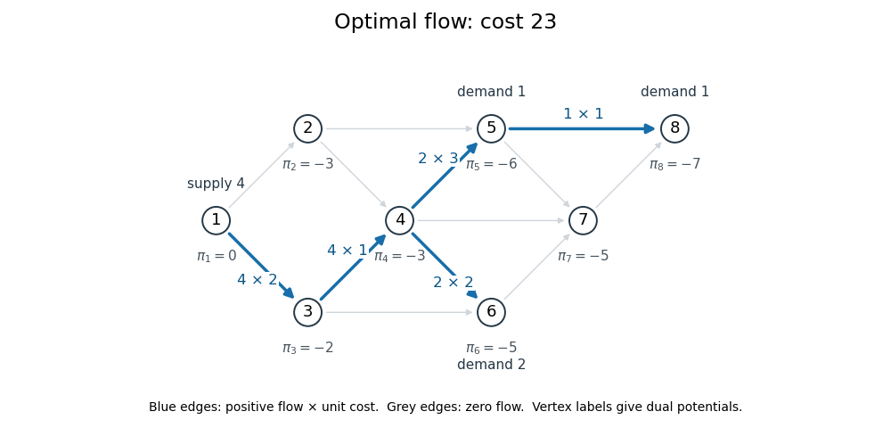
On the dashed spanning tree, the nonzero flows arewith $f_{78}=0$ and all non-tree flows zero. The tree balances give supply four at vertex $1$, demands one at $5$ and $8$, and demand two at $6$. Its cost is $25$.

Choose ${\pi }_1=0$ and make the tree network reduced costs zero. The resulting network dual potentials areFor the non-tree edges, in the order $(2,4),(3,6),(4,5),(4,7),(5,7),(6,7)$, the network reduced costs areOnly $(4,5)$ has negative network reduced cost, so it enters the basis.

Adding this edge to the tree creates the graph cycle $4\to 5\to 2\to 1\to 3\to 4$. Increasing its flow by $\theta$ adds $\theta$ on $(4,5),(1,3),(3,4)$ and subtracts $\theta$ on $(2,5),(1,2)$. These signed changes preserve every flow balance. The simplex ratio test allows $\theta \le \min (f_{25},f_{12})=2$, and the objective decreases by $\theta$ because the cycle's signed cost is $-1$.

Take $\theta =2$ and remove $(2,5)$ from the basis. The other tied edge $(1,2)$ remains a zero-flow basic edge; this is a legitimate degenerate tree basis and requires no extra pivot. The new flow isIts cost is $8+4+6+4+1=23$. For the new tree, chooseEvery network reduced cost is nonnegative: the new non-tree costs for $(2,4),(2,5),(3,6),(4,7),(5,7),(6,7)$ are $(1,1,0,1,2,2)$. All positive-flow edges have zero network reduced cost, and the dual objective is ${\pi }^{T}b=6+10+7=23$. Thus complementary slackness gives

P is the class of decision problems decided by a deterministic algorithm in time polynomial in the encoded input length. NP is the class whose yes-instances have complexity certificates of polynomial length that a deterministic algorithm verifies in polynomial time.

A decision problem is NP-complete if it belongs to NP and is NP-hard: every problem in NP admits a polynomial-time many-one reduction to it. Such a reduction maps an instance $I$ to an instance $R(I)$ in polynomial time and satisfies $I$ is a yes-instance if and only if $R(I)$ is a yes-instance. Membership in NP and NP-hardness are both required.

Run breadth-first search separately in every component of the undirected graph. Give a starting vertex colour zero and each newly discovered neighbour the opposite colour. Reject if an edge joins two vertices with the same assigned colour; otherwise accept after all components have been explored.

If the algorithm accepts, its assignments constitute a graph colouring with two colours. If it rejects, the two search-tree paths and the conflicting edge contain an odd cycle, on which alternating two colours cannot close consistently. Equivalently, a valid graph colouring with two colours fixes the parity of every path from a component's root, so the detected conflict is impossible in a two-colourable graph. The breadth-first search work is $O(|V|+|E|)$ with adjacency lists. ThereforeThis is also the two-colourability criterion for bipartite graphs.

The displayed graph consists of three graph triangles sharing the vertex $v$. In a graph colouring with three colours, every graph triangle uses all three colours. The edge $tf$ and the edges $tv,fv$ therefore force $c(t),c(f)$ to be the two colours different from $c(v)$. Likewise the graph triangle $vxy$ forces $c(x),c(y)$ to be those same two colours. The third graph triangle imposes no further restriction on these four vertices. HenceBoth two-element sets and their union have cardinality two. This is a Boolean-pair colouring gadget: after fixing a palette graph triangle, the pair $x,y$ encodes opposite truth values.

Name the upper graph triangle's vertices $a,b,c$, where $b$ is adjacent to $x$ and $c$ to $y$. Name the middle left vertex $d$ and the lower right vertex $e$. Then $a$ is adjacent to $d$, the lower graph triangle is $d,t,e$, and $e$ is adjacent to $z$.

Suppose $x,y,z$ all have colour $F$, while $t$ has a different colour $T$; denote the third colour by $B$. In the upper graph triangle, $b$ and $c$ cannot have colour $F$ and are adjacent, so they have colours $T,B$ in some order and $a$ has colour $F$. In the lower graph triangle, $e$ is adjacent to both $t$ and $z$, forcing $e$ to have colour $B$, and then $d$ must have colour $F$. But the edge $ad$ now has equal-coloured endpoints, a contradiction. ThusFor the three-colour clause gadget used in a reduction, one also needs the converse extension property for Boolean-coloured inputs. With $t=T$ and $x,y,z\in \{T,F\}$, every tuple other than $(F,F,F)$ extends. If $x=T$, take $(a,b,c,d,e)=(T,F,B,F,B)$; this works regardless of $y,z$. If $x=F,y=T$, take $(T,B,F,F,B)$. Finally, if $x=y=F,z=T$, take $(F,T,B,B,F)$. Each assignment satisfies every edge. Therefore this three-colour clause gadget realizes exactly a three-input disjunction on Boolean inputs.

The three-colourability problem belongs to NP: a colour assignment is a polynomial-length complexity certificate, and all edges can be checked in $O(|V|+|E|)$ time.

For NP-hardness, reduce 3-SAT to the three-colourability problem. Start with a palette graph triangle with vertices $T,F,B$. Its colours are necessarily distinct, and name them by these vertices. For each Boolean variable $u$, add vertices $u,\bar{u}$, join them to each other, and join each to $B$. The graph triangle $B,u,\bar{u}$ is the forcing component of the Boolean-pair colouring gadget, so the two literal vertices receive opposite colours $T,F$.

For each Boolean clause, attach a fresh copy of the three-colour clause gadget, identify its $t$ with the palette vertex $T$, and identify its three input vertices with the Boolean clause's Boolean literal vertices. Copies share only palette or literal vertices. A Boolean clause with one or two Boolean literals is padded to three by repeating a literal; an empty Boolean clause can be mapped immediately to the uncolourable graph $K_4$.

Any graph colouring with three colours gives a truth assignment by reading colour $T$ as true. The three-colour clause gadget forbids three false inputs, so every Boolean clause is satisfied. Conversely, any satisfying truth assignment colours the literal pairs, and the extension property proved above independently colours the fresh auxiliary vertices of each clause. Thus the entire graph is three-colourable exactly when the formula is satisfiable.

There are $3+2n+5m$ vertices for $n$ variables and $m$ nonempty padded clauses, and $O(n+m)$ edges. The construction is a polynomial-time many-one reduction. Using the permitted NP-completeness of 3-SAT, we obtain

Form a bipartite graph with one vertex for each row and one for each column, putting an edge $ij$ exactly where $a_{ij}>0$. For a set $S$ of row vertices, let $N(S)$ be its neighbouring column vertices. Since $A$ is a doubly stochastic matrix,The Hall marriage theorem therefore supplies a perfect matching. Its incidence entries define a permutation matrix $P$ supported on the positive entries of $A$, hence on the ones of $B$. Entrywise $P\le B$, so

The preceding perfect matching gives a permutation matrix $P$ supported on the positive entries of $A$. LetIf $\alpha =1$, every row's selected entry is one and all other entries vanish, so $A=P$. Otherwiseis a doubly stochastic matrix with strictly fewer positive entries. Induct on the number of positive entries: the base case has exactly $n$ positive entries and is a permutation matrix. By induction, write $A^{\prime }={\sum }_i{\beta }_i{P}_i$ as a convex combination. Thenis another convex combination, with nonnegative coefficients summing to one. ThusThis constructive proof of the Birkhoff-von Neumann theorem is Birkhoff decomposition by support matchings.

For an explicit algorithm, keep an unnormalized residual $R$, initially $A$, whose row and column sums all equal a common mass $\tau$, initially one. While $\tau >0$, find a perfect matching in its positive support, form its permutation matrix $P$, and subtract $\alpha P$, where $\alpha$ is the smallest selected entry. Record $(\alpha ,P)$ and replace $\tau$ by $\tau -\alpha$.

If the residual mass is positive, the same proof of the Hall marriage theorem condition applies after division by $\tau$. Every subtraction removes at least one positive entry and creates no new positive entries. Before the last subtraction, any positive-mass residual has at least $n$ positive entries; the last step removes all its entries. If $r$ is the initial number of positive entries, thenSince the residual ultimately vanishes, summing the recorded subtractions gives $A=\sum {\alpha }_i{P}_i$, and the row sums give $\sum {\alpha }_i=1$.

A perfect matching can be found by at most $n$ searches for an augmenting path in a matching, each costing $O(n^2)$ in a graph with at most $n^2$ edges. Thus each iteration costs $O(n^3)$, including forming the support and updating the residual, and there are $O(n^2)$ iterations. HenceThis bound uses exact real arithmetic. For rational input, a common denominator lets all residual subtractions be performed on integers of polynomial bit length, giving a polynomial bit-time implementation as well.

Apply positive affine payoff transformations, if necessary, so both payoff matrices have strictly positive entries. Such transformations preserve best responses and Nash equilibria. The Lemke-Howson algorithm uses unnormalized nonnegative strategy vectors and slack variables satisfyingThus its two polytopes are $\{x\ge 0:Q^{T}x\le 1\}$ and $\{y\ge 0:Py\le 1\}$. A label $i\le m$ occurs when $x_i=0$ or $r_i=0$; a label $m+j$ occurs when $y_j=0$ or $s_j=0$. The complementary pivoting path drops one label from the artificial zero pair and resolves each duplicated label until all labels return.

Terminate at a completely labelled pair other than the artificial zero pair. This is equivalent to complementary slacknessA nonzero completely labelled pair has both vectors nonzero: if $x=0$, then $s=1$ forces $y=0$, and the converse is analogous. Normalize to mixed strategiesThe inequalities $Py\le 1$ imply that every row payoff against $q$ is at most $1/(1^{T}y)$, with equality on every row receiving positive probability in $p$. Thus $p$ is a best response to $q$. Likewise $q$ is a best response to $p$ using $Q^{T}x+s=1$. Hence $(p,q)$ is a Nash equilibrium. Nondegeneracy of a bimatrix game ensures the usual complementary pivoting path has a unique continuation after the label choice.

In the first tableau the basis is $(x_2,s_5,x_1)$, givingThe second basis is $(r_1,y_6,r_3)$, giving $y=(0,0,1/4)$ and $r=(3/4,0,1/4)$. This pair is not yet a Nash equilibrium: label $1$ is missing and label $4$ is duplicated.

Resolve the duplicate by bringing $y_4$ into the second tableau. Its column is $(3/4,1/4,9/4{)}^T$, so the simplex ratio test givesVariable $r_3$ leaves, givingNow label $3$ is duplicated. Bring $x_3$ into the first tableau; its column is $(0,3,1{)}^T$. The positive-entry ratios are $(2/3)/3=2/9$ and $(1/9)/1=1/9$. Thus $x_1$ leaves, givingAll labels are now present and $x_i{r}_i=y_j{s}_j=0$. Each unnormalized strategy has total mass $1/3$, so the Lemke-Howson algorithm produces

Row operations multiply each original tableau equation by an invertible matrix. The slack variable block therefore records that matrix and allows the original payoff matrix to be recovered without guessing.

From the first tableau, let $X$ be the coefficient block of $x$ and $S$ that of $s$. Since its original equations were $Q^{T}x+s=1$, we have $Q^T=S^{-1}X$. HeresoFor the second tableau, writing its $y$ and $r$ blocks as $Y,R$, the original equations $Py+r=1$ give $P=R^{-1}Y$. We obtainThus a representative pair of payoff matrices isBoth reconstructed right-hand sides are $1$, as a check on the tableau normalization. Independent transformations $P\mapsto aP+b11^T$, $Q\mapsto cQ+d11^T$, with $a,c>0$, preserve best responses and hence identify the same strategic solution up to positive affine payoff transformations.

Directly,The supports of $x^{\prime }$ and $y^{\prime }$ lie entirely among their respective best-response coordinates, confirming the Nash equilibrium found above. Since this representative is a symmetric bimatrix game, swapping the players' strategies preserves the Nash equilibrium conditions. Explicitly, $P{x}^{\prime }=(3,2,3{)}^T$ is maximized on the support of $y^{\prime }$, and $Q^T{y}^{\prime }=P{y}^{\prime }=(1,3,3{)}^T$ is maximized on the support of $x^{\prime }$. Therefore