Past exam of the mathematics course of the University of Cambridge / 2015 / iii / Paper 43 (Quantum Field Theory)

Use natural units and the Minkowski metric $\eta =\mathrm{diag}(1,-1,-1,-1)$. A real scalar field assigns a real variable $\varphi (t,\mathbf{x})$ to each spatial point. Its Lagrangian density can be taken to beThe principle of stationary action gives the Euler-Lagrange equation $\square \varphi +V^{\prime }(\varphi )=0$. With $V(\varphi )=m^2{\varphi }^2/2$, this is the Klein-Gordon equation. An additional nonlinear part of $V$ describes interactions.

The canonical momentum is $\pi =\partial \mathcal{L}/\partial \dot{\varphi }=\dot{\varphi }$. The Legendre transform in mechanics gives the canonical Hamiltonian density of a real scalar fieldThe Hamiltonian equations $\dot{\varphi }=\pi$ and $\dot{\pi }={\nabla }^2\varphi -V^{\prime }(\varphi )$ recover the same field equation. In canonical quantization, the fields become operators satisfying the equal-time canonical commutation relationsA spatial lattice makes the analogy with many coupled quantum-mechanical coordinates precise. Each lattice field value is a coordinate, with its own conjugate momentum. The path integral is another representation of the same quantum evolution.

To see its origin, first consider one coordinate with $H=p^2/(2M)+V(q)$. Split a time interval into $N$ steps of length $\epsilon$ and insert position and momentum resolutions of the identity. The short-time kernel isMultiplying the kernels and integrating over intermediate positions gives the phase-space path integralThe endpoints of $q$ are fixed. The momentum integrals are Gaussian integrals; completing the square produces the configuration-space path integralAt finite slicing its normalization contains $(M/(2\pi i\epsilon ){)}^{N/2}{\prod }_{j=1}^{N-1}d{q}_j$. This fixes the composition law and the initial delta-function kernel. One sums over all paths, not merely solutions of the classical equation. Restoring $\hslash$ replaces the weight by $e^{iS/\hslash }$; stationary phase explains the emergence of classical trajectories.

For the field, use scalar field configuration eigenstates $|\phi ⟩$, satisfying $\hat{\varphi }(\mathbf{x})|\phi ⟩=\phi (\mathbf{x})|\phi ⟩$. Insert their completeness relations on every time slice. This givesThe endpoint field configurations are fixed. Integrating the Gaussian momentum variables leaves the scalar field path integral $\mathcal{N}\int \mathcal{D}\varphi e^{iS[\varphi ]}$. The functional measure means a regulated product over the field variables. A spacetime lattice or another ultraviolet cutoff makes this product finite before the continuum limit; interacting continuum calculations may require renormalization. The oscillatory Minkowski weight is an amplitude, not a positive probability density.

For vacuum expectation values, the boundaries must select the vacuum rather than arbitrary field configurations. Long imaginary-time evolution suppresses excited states: $e^{-TH}|n⟩=e^{-T{E}_n}|n⟩$, so after normalization only the lowest-energy component remains as $T\to \infty$. This is vacuum projection by imaginary time. The corresponding Feynman i-epsilon prescription in the real-time integral specifies the vacuum boundary conditions and the poles of the propagator. With $t=-i\tau$, the Euclidean path integral has the weight $e^{-S_E}$, whereIt is often a useful regulated starting point; analytic continuation returns the vacuum time-ordered quantities.

Introduce a classical source $J(x)$ and define the normalized vacuum generating functionalwith the same vacuum prescription in numerator and denominator. A functional derivative brings down $i\varphi (x)$. The order of the time slices makes the operator insertion time-ordered. Thus source differentiation inserts time-ordered field operators:The denominator removes vacuum diagrams and gives normalized expectation values. It is essential that these are time-ordered products; differentiating this vacuum functional does not directly give every possible operator ordering.

The free theory illustrates the method. Its quadratic kernel is $K=-\square -m^2$ with the vacuum pole prescription, and completing the square gives the Gaussian evaluation of a free scalar generating functionalTwo source derivatives give ${\Delta }_F=⟨\Omega |T\{\hat{\varphi }(x)\hat{\varphi }(y)\}|\Omega ⟩$. Higher derivatives give all pairings, the content of Wick theorem. For an interaction $S_{\mathrm{int}}$, one may use path-integral perturbation by source derivatives:Expanding this expression generates Feynman diagrams and their Wick contractions. The connected generating functional $W[J]=-i\log Z[J]$ retains connected contributions; in particular $\delta W/\delta J=⟨\varphi {⟩}_J$. These functionals turn the computation of field-operator expectations into source differentiation of an ordinary regulated integral.

Use the momentum-space Feynman rules with the scalar Feynman propagator $i/(p^2-m^2+i0)$. The four-leg vertex of a factorial-normalized scalar interaction has weight $i\lambda$ for the positive interaction sign printed here. There are $4!$ Wick contractions assigning four external legs to its four fields, cancelling the factorial in its coefficient. A negative interaction sign would give $-i\lambda$; its squared tree amplitude is the same.

At each vertex include $(2\pi {)}^4{\delta }^4(\sum p)$ with all incident momenta taken incoming. Assign an internal momentum to each line and integrate each independent loop with $\int d^4\ell /(2\pi {)}^4$. Divide a graph by its Feynman-diagram symmetry factor, sum the graphs at the chosen order, and omit disconnected vacuum graphs from normalized amplitudes. For an S-matrix element, amputate external propagators and put the external momenta on shell as in the LSZ reduction formula; the external one-particle residues are one at tree level.

Define the invariant amplitude by the relativistically normalized matrix elementwith $⟨p|p^{\prime }⟩=2E_{\mathbf{p}}(2\pi {)}^3{\delta }^3(\mathbf{p}-{\mathbf{p}}^{\prime })$. The lowest-order connected four-point graph is one contact vertex:There is no exchange graph at this order because there is no three-field interaction.

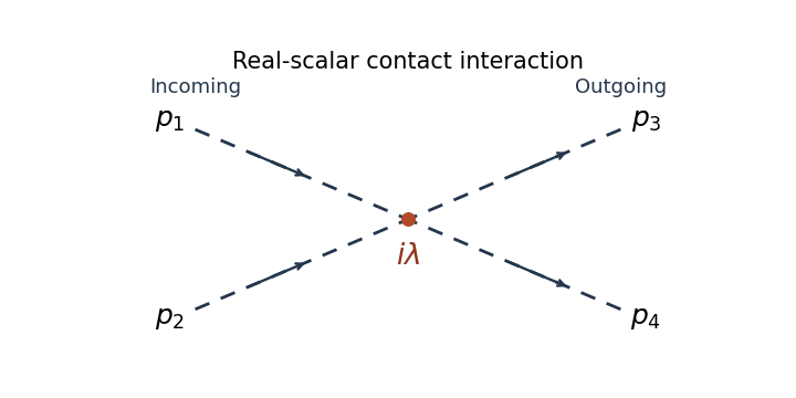
For the elastic scattering from a quartic scalar contact interaction, write $\sqrt{s}$ for the total centre-of-mass energy and $E_p=\sqrt{s}/2$ for the energy of each incoming particle. The incoming and outgoing spatial momentum magnitudes both equal $k=\sqrt{E_p^2-m^2}$, with $E_p>m$. The invariant incident flux isThe Lorentz-invariant phase-space measure for two outgoing particles isIn the centre-of-mass frame, the spatial delta function sets ${\mathbf{p}}_4=-{\mathbf{p}}_3$, while the energy delta function has radial derivative $2k/E_p$. Therefore the relativistic two-body phase space satisfiesThe two outgoing real-scalar particles are identical. Integrating over the full solid angle counts each unordered pair twice, so include the identical final-state symmetry factor $1/2!$. This givesThis is isotropic. When $E$ denotes each particle's energy, $s=4E^2$ and the full-sphere event density is ${\lambda }^2/(512{\pi }^2{E}^2)$. If $E$ denotes the total energy of the pair, $s=E^2$ and it is ${\lambda }^2/(128{\pi }^2{E}^2)$. Stating the answer in $s$ removes that energy-label ambiguity.

An equally valid angular convention selects one outgoing particle in a hemisphere, so each event is represented once. In that convention omit $1/2!$ and use $d\sigma /d\Omega ={\lambda }^2/(64{\pi }^{2}s)$ on the hemisphere, or ${\lambda }^2/(256{\pi }^2{E}_p^2)$. Both conventions give ${\sigma }_{\mathrm{event}}={\lambda }^2/(32\pi s)$ at this order. The identical-state factor concerns counting final states and is separate from the vertex factorial.

Use signature $(+---)$ and take the covariant spatial components $A_i$ as canonical coordinates. The canonical quantization of the electromagnetic field begins with the canonical momentaThus the primary momentum constraint of the electromagnetic potential is ${\Pi }^0=0$: $A_0$ has no independent velocity. The Hamiltonian obtained by the Legendre transform in mechanics, up to a boundary term, isPreserving the primary constraint requires the Gauss law constraint in gauge theory, ${\partial }_i{\Pi }^i=0$. It also follows by varying $A_0$. These are two first-class constraints; they generate the gauge freedom and remove two canonical pairs from the four potential components. The reduced phase space has four dimensions per spatial mode, hence two propagating photon degrees of freedom.

Impose Coulomb gauge, ${\partial }_i{A}_i=0$. With no charges, Gauss's law then gives ${\nabla }^2{A}_0=0$; vanishing boundary conditions set $A_0=0$. This is radiation gauge. The remaining components are transverse and obey the massless wave equation. Let ${ϵ}_i^{(r)}(\mathbf{k})$, $r=1,2$, be orthonormal transverse polarization vectors. Their photon polarization completeness relation isThe canonical transverse photon field is the Hermitian operatorwhereThe field and its conjugate momentum have the transverse equal-time commutatorThis is the quantized reduced bracket, or equivalently the Dirac bracket after imposing the constraints and gauge conditions. The normal-ordered Hamiltonian is ${\sum }_r\int d^{3}k{\omega }_{\mathbf{k}}{a}_r^{†}{a}_r/(2\pi {)}^3$. Its excitations are photons; circular combinations of the two transverse polarizations have helicity $+1$ and $-1$. The scalar and longitudinal potential components do not create additional physical photons.

The Feynman propagator is the vacuum expectation of a time-ordered product. The mode expansion directly gives the radiation-gauge photon propagator, with $z=x-y$:The first expression comes from the creation-annihilation commutator; the second is its contour-integral representation. The positive-energy pole lies below the real axis and the negative-energy pole above it. In this reduced free-field description, the temporal operator is zero. A photon propagator must specify its gauge; the spatial transverse propagator is not the same tensor as the covariant four-potential propagator.

For the commonly used covariant form, add the gauge fixing term $-({\partial }_{\mu }{A}^{\mu }{)}^2/(2\xi )$. The resulting Fourier-space kinetic operator isThe inversion of the gauge-fixed Maxwell kinetic operator gives $K^{\mu \nu }{D}_{\nu \rho }^F=i{\delta }^{\mu }{}_{\rho }$. In Feynman gauge, $\xi =1$, the photon propagator isEquivalently, $\square D_{\mu \nu }^F=i{\eta }_{\mu \nu }{\delta }^4(x-y)$ with the vacuum pole prescription. For general $\xi$, the momentum-space numerator is ${\eta }_{\mu \nu }-(1-\xi )k_{\mu }{k}_{\nu }/(k^2+i0)$.

A covariant canonical realization uses four polarization oscillators with $[a_r,a_s^{†}]=-(2\pi {)}^3{\eta }_{rs}{\delta }^3(\mathbf{k}-{\mathbf{k}}^{\prime })$. The resulting indefinite inner product is auxiliary. In Gupta-Bleuler quantization, impose $({\partial }_{\mu }{A}^{\mu }{)}^{(+)}|\mathrm{phys}⟩=0$ and take the Gupta-Bleuler null-state quotient. The scalar-longitudinal combination is thereby removed from the physical state space, leaving the same two transverse photon states. Thus the four-component Feynman-gauge numerator does not imply four physical polarization states.

Use gamma matrices satisfying the Clifford algebra relation $\{{\gamma }^{\mu },{\gamma }^{\nu }\}=2{\eta }^{\mu \nu }$, with ${\gamma }^{0†}={\gamma }^0$ and ${\gamma }^{i†}=-{\gamma }^i$. The Dirac adjoint is $\bar{\Psi }={\Psi }^{†}{\gamma }^0$. Take the Dirac actionIt differs from the manifestly Hermitian form with $(i/2)\bar{\Psi }{\gamma }^{\mu }{\overleftrightarrow{\partial }}_{\mu }\Psi$ only by a boundary term. Treat $\Psi$ and $\bar{\Psi }$ as independent variables when applying the principle of stationary action. Varying $\bar{\Psi }$ givesVarying $\Psi$ and integrating by parts gives the adjoint Dirac equation, $i({\partial }_{\mu }\bar{\Psi }){\gamma }^{\mu }+m\bar{\Psi }=0$. Multiplying the Dirac equation by $i{\gamma }^{\nu }{\partial }_{\nu }+m$ also gives $(\square +m^2)\Psi =0$, so its dispersion relation is Lorentz invariant.

For a Lorentz transformation $x^{\prime }=\Lambda x$, the field transforms in the Spinor representation of the Lorentz group:Since ${\partial }_{\mu }^{\prime }=({\Lambda }^{-1}{)}^{\nu }{}_{\mu }{\partial }_{\nu }$, this identity gives the Lorentz covariance of the Dirac operator:Thus every solution is carried to another solution. The field is a spinor rather than a four-vector; the transformation of the gamma matrices supplies the necessary covariance. The Dirac action is Lorentz invariant because its integrand is a scalar and $d^{4}x$ is invariant.

For electric charge $q$, use the gauge covariant derivative $D_{\mu }={\partial }_{\mu }+iq{A}_{\mu }$. The minimal electromagnetic coupling of a Dirac field isThe local gauge transformations in this convention areDirect substitution gives $D_{\mu }^{\prime }{\Psi }^{\prime }=e^{-iq\alpha }{D}_{\mu }\Psi$, which proves gauge covariance of the charged Dirac equation. The mass and kinetic terms are invariant, and $F_{\mu \nu }^{\prime }=F_{\mu \nu }$, so the full action has gauge invariance. The conserved current is $j^{\mu }=q\bar{\Psi }{\gamma }^{\mu }\Psi$. It transforms as a four-vector under Lorentz transformations, and varying $A_{\mu }$ gives ${\partial }_{\nu }{F}^{\nu \mu }=j^{\mu }$.

To make the infinitesimal spinor transformation explicit, write ${\Lambda }^{\mu }{}_{\nu }={\delta }^{\mu }{}_{\nu }+{\omega }^{\mu }{}_{\nu }$ with ${\omega }_{\mu \nu }=-{\omega }_{\nu \mu }$. DefineThe Lorentz generators from gamma-matrix commutators have precisely the needed algebra: $[{\sigma }^{\mu \nu },{\gamma }^{\rho }]=2i({\eta }^{\nu \rho }{\gamma }^{\mu }-{\eta }^{\mu \rho }{\gamma }^{\nu })$, which verifies $S^{-1}{\gamma }^{\rho }S={\gamma }^{\rho }+{\omega }^{\rho }{}_{\nu }{\gamma }^{\nu }$ to first order. The infinitesimal transformation of a Dirac field is thereforeAt the same coordinate argument, the orbital change must also be included:Both formulas describe the same transformation; their arguments differ.

Finally, the gamma adjoint identities imply ${\sigma }^{\mu \nu †}={\gamma }^0{\sigma }^{\mu \nu }{\gamma }^0$ and hence the pseudo-unitarity of the spinor Lorentz representation, $S^{†}{\gamma }^{0}S={\gamma }^0$. It follows thatThus the Dirac scalar bilinear $\bar{\Psi }\Psi$ is a Lorentz scalar. Infinitesimally the spin terms in $\delta (\bar{\Psi }\Psi )$ cancel; at fixed coordinates only the ordinary scalar orbital transformation remains.