Write the radial velocity as , allowing for accretion flow, and let be the squared adiabatic sound speed. The steady continuity equation, radial Euler equations for an inviscid fluid and entropy advection equation giveOn a nonzero smooth flow branch, the polytropic equation of state is with constant . Thus the two useful first integrals for spherically symmetric adiabatic flow areHere is the signed mass flux and is the Bernoulli function. The specific enthalpy is ; the prescribed Newtonian gravitational potential has no contribution from the gas's own gravity. Eliminating the density derivative using mass conservation gives the differential formThis sonic point equation displays both the singular coefficient and the numerator that must vanish for a smooth transonic branch.
At a finite smooth sonic point , the equation from (a) requiresSet and . Substitution into the Bernoulli function givesAn inflow from a warm reservoir at infinity has ; an outflow reaching infinity has . Therefore a nondegenerate transonic spherical flow in a power-law potential requiresFor the usual range , the critical adiabatic exponent for spherical power-law flow is consequentlyThe printed assumption also permits . In that range the boxed inequality holds for every finite : there is no finite upper bound. Equivalently, take for . Extending the rational expression beyond would give an incorrect restriction.
The strict inequality also follows from local sonic-point slope discriminant analysis, including the potentially cold zero-energy endpoint. Put . Since mass conservation implies , differentiating the sonic point equation at yieldsIts discriminant is . Moreover, the logarithmic Mach number derivative at the sonic point isA genuine crossing has two distinct branches and a nonzero derivative. At equality the crossing degenerates. In particular, for and , mass conservation and the polytropic equation of state make the Mach number constant along the scale-invariant solution; a solution that is sonic there is sonic everywhere, rather than crossing an isolated sonic point.
Use the positive mass accretion rate , and retain , . Define , which is positive under the condition in (b). Matching the Bernoulli function to the reservoir and using the polytropic equation of state givesThe transonic spherical accretion rate in a power-law potential is thereforeThe combination has dimensions of length to the power , so this expression has dimensions of mass per time. The sonic point selects the flux that connects the subsonic reservoir to the inward supersonic transonic branch.
For the endpoint limits of power-law spherical accretion, hold fixed. As , , so . HenceThis is also obtained directly from an isothermal equation of state: the Bernoulli function becomes , so . For , , it recovers the isothermal Bondi accretion rate.
For , and means . Since ,ThusThe finite limiting flux accompanies and ; it does not assert a finite-radius sonic point at the endpoint. For this is the familiar limit .
For completeness, the printed range has the endpoint . At , and the flux is independent of , namely . For , and , so as . These are the corresponding extended endpoint limits.
The solenoidal constraint on the magnetic field reduces to . Locally, or globally in a simply connected cross-section, it permits a Cartesian magnetic flux function satisfyingThe transverse magnetic field lines are contours of , because . The independent component supplies the twist of the flux tube; it is not restricted by the solenoidal constraint.
For the Lorentz force, take the curl explicitly:Its cross product with has transverse components and component . ConsequentlyThe term is the transverse gradient of the magnetic pressure associated with the axial field, while the other terms include magnetic tension.
In magnetostatics, . The plane-parallel Newtonian gravitational potential and all thermodynamic fields are independent of , so the component of the Lorentz force must vanish:Away from a null of , this says that is constant along each connected contour of the Cartesian magnetic flux function. Thus, on a regular flux region,This statement is local; disconnected contours with the same numerical flux label need not share one global function without the usual flux-tube connectivity assumption.
Since , the transverse magnetostatic equilibrium equation becomesThis is a Cartesian magnetostatic flux-function equilibrium. Projecting it along a transverse magnetic field line gives hydrostatic balance along that line; projecting across the line balances the gas pressure and weight against magnetic pressure and magnetic tension.
The MHD induction equation can be written in material form asIts component immediately givesFor the Cartesian magnetic flux function, the components of the MHD induction equation, or the component of the magnetic vector potential equation, giveThe additive function of time in has no effect on . Choose this gauge so that . Then the flux label is materially conserved:This is magnetic flux freezing in the two-dimensional geometry.
To prove the absence of axial motion, construct an invariant solution with . Along each Lagrangian trajectory, is fixed, and the assumed divergence givesThus remains a function of and time alone. Its gradient stays parallel to , so the component of the Lorentz force remains zero. The axial momentum equation isbecause . With initially, it remains zero. Hence neither axial force nor axial motion is generated. This flux-surface preservation during magnetic-tube expansion argument assumes the smooth ideal evolution for which the initial-value problem is unique; the particular in-plane rising motion need not be calculated.
Use , , and a prime for . For the plane-parallel magnetohydrodynamic flow with imposed shear, , whileThe solenoidal magnetic field constraint gives . The component of the MHD induction equation then gives . Thus is constant in both space and time.
Use the magnetic tension and magnetic pressure decompositionThe continuity equation and momentum equation now reduce toThe transverse components of the MHD induction equation areThe terms involving respectively accelerate the flow across the imposed shear flow and wind the transverse magnetic field. The closure is the isothermal equation of state , as printed in the PDF.
The logarithmic density term is the barotropic fluid energy for , rather than the thermodynamic heat content of an isolated gas. DefineFor any scalar , the continuity equation implies . Therefore , , and dotting the momentum equations with givesThe MHD induction equation gives the complementary magnetic energy balanceAdding these two identities, and collecting the product derivatives, yields the barotropic magnetic energy equationHere . The two stress terms in describe magnetohydrodynamic shear work: the maintained background shear flow can supply energy to, or remove energy from, the perturbation flow and magnetic field. The sign depends on the off-diagonal total stress; this is why the energy excluding the background shear flow is not generally conserved. Changing merely adds a constant multiple of the conserved density to and the corresponding mass flux to , leaving unchanged.
For a steady flow, mass conservation gives and . Define the Alfvén velocity and . Combining the horizontal momentum and MHD induction equations without dividing by givesDot these identities with and , respectively:The vertical momentum equation and the isothermal equation of state giveMultiply by and eliminate the magnetic derivative to obtainNo division by was needed in deriving this necessary relation.
The magnetosonic critical speeds in the direction areThe plus sign gives the fast magnetosonic wave speed and the minus sign the slow magnetosonic wave speed. Thus the differential coefficient is . A smooth outflow proceeding from below both speeds to above both must normally pass through both magnetosonic critical speeds. At each crossing, the right-hand side must also vanish; this is the regularity at a magnetosonic point condition. The derivative coefficient changes sign at each nondegenerate crossing. For and , the driving term must be positive below the slow point, negative between the points and positive above the fast point.
The Alfvén speed component satisfies . With downward gravity , the gravitational term is consequently nonnegative at the slow point and nonpositive at the fast point. The magnetohydrodynamic shear work contribution must balance it at each point, and can provide the upward driving needed to pass the fast point. For and strictly positive , generic separated slow and fast points cannot satisfy the required zero numerator; special vanishing-gravity or coincident-speed cases need separate treatment.
There is also Alfvén-point compatibility in a plane-parallel sheared flow. At , the original transverse equations requireThese restrictions are not generally visible as a zero of the scalar differential coefficient, which there equals . In particular, a strictly accelerating regular solution must have at that point. The scalar relation is therefore a necessary wind equation, not a substitute for regularity of all the original ideal magnetohydrodynamic equations. Degenerate cases such as a purely longitudinal magnetic field can merge characteristic speeds and reduce the number of distinct critical conditions.
Use the fluid displacement , with velocity perturbation . Denote Eulerian perturbations by and the corresponding Lagrangian pressure perturbation by . For adiabatic perturbations, the linearized mass conservation, momentum, adiabatic equation of state and Poisson equation areThese self-gravitating adiabatic displacement equations retain the perturbation of the star's own Newtonian gravitational potential. In the uniform-density interior, , , and . The dynamical frequency of a uniform-density star sets the natural timescale. For a normal mode with time factor , replace by . The requested interior analysis needs no surface or exterior matching conditions.
The spatial factor is a regular solid harmonic. Besides the Laplace equation , homogeneity gives . The divergence of the fluid displacement isDefine the scalar dilation amplitude ; this is the quantity denoted in the question, not the notation for a Lagrangian pressure perturbation. Then mass conservation gives .
The equilibrium pressure gradient and homogeneity identity giveConsequently the adiabatic equation of state yieldsFor the force equations, the product rule givesEquating the coefficients of and in the self-gravitating adiabatic displacement equations givesFinally, applying the Laplacian to the gravitational perturbation givesso the Poisson equation becomesThese are the required interior equations for uniform-density stellar oscillation.
There is a radial degeneracy at : is spatially constant and , so the displacement is independent of . The second force equation then cannot be inferred by equating independent vectors. For nonzero it may be imposed as an auxiliary definition of , but it is not an additional physical radial equation. At zero frequency the radial equations should be used directly. This distinction matters for interpreting the zero factor in (c).
For the polynomial stellar-mode coefficient reduction, write the highest coefficients asSet , and . The highest powers in the equations of (b) giveThe factor follows from ; the positive term comes from the highest, negative coefficient of the equilibrium pressure.
For , the final spectrum found below has . Eliminating first givesThe remaining pressure relation isA nontrivial leading coefficient has , soThusor, in dimensional form,
For the printed stability continuation, define . The two branches for nonradial stellar oscillations areFor every , their product is . Therefore one branch oscillates and the other grows exponentially, for every positive . With the chosen time dependence, gives and growth rate . Increasing does not remove this nonradial instability. At large or large , is a stiff compressive branch, while is a slower unstable buoyancy branch.
The buoyancy frequency supplies the physical explanation. The background density has zero gradient, but pressure decreases outward:The specific entropy of the perfect gas decreases outward, because does. An adiabatically displaced fluid parcel therefore experiences destabilizing buoyancy. The model has convective instability of a uniform-density star, even when its radial compression modes are stable. The divergence of this expression at the zero-pressure surface also reflects the artificial equilibrium; the interior negative sign is already decisive.
For , the formal quadratic factors asThe physical radial displacement has no component. Using its equations directly givesIndeed , , and yield this result directly in the radial momentum equation. The extra identically zero factor in the two-component determinant need not represent an independent radial mode, since is redundant when .
The lowest allowed degree, , has . Hence all these radial modes are stable for ; the fundamental radial mode is marginal at and unstable below it. Higher have their individual thresholds . These radial stability of a uniform-density star thresholds coexist with nonradial convective instability. They are conclusions within the polynomial interior family assumed in the question; no boundary-condition quantization is being asserted.
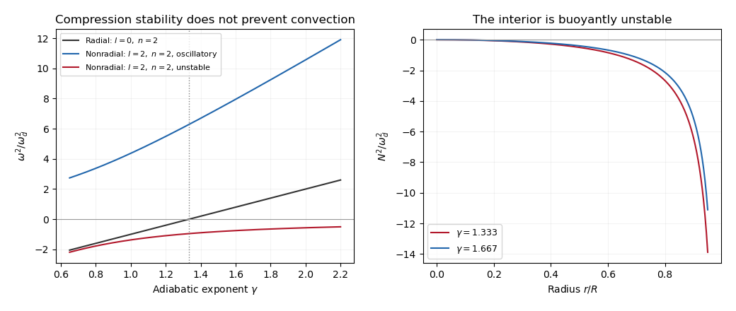
Radial and nonradial squared mode frequencies and the negative buoyancy frequency of a uniform-density gas star
. Details. 
Articles by others on the same topic
There are currently no matching articles.