Past exam of the mathematics course of the University of Cambridge / 2018 / iii / Paper 311 (Black Holes)

The action contains neither $\dot{N}$ nor ${\dot{N}}^i$, so their conjugate momentum vanishes. They impose constraints rather than independent evolution equations: after the Legendre transform in mechanics, the lapse function and shift vector are Lagrange multipliers in the Hamiltonian formulation of general relativity.

Use precisely the paper's sign convention for extrinsic curvature, $K_{ij}=({\dot{h}}_{ij}-D_i{N}_j-D_j{N}_i)/(2N)$. At fixed $h_{ij},N,N^i$,Consequently the canonical momentum of the spatial metric isThis is a weight-one tensor density, with indices raised and lowered using $h_{ij}$. Its trace and inverse relation areThe sign of $K_{ij}$ used here is opposite to the convention in extrinsic curvature of a spatial hypersurface; mixing the two conventions would reverse the momentum formula.

In the paper's convention, ${\dot{h}}_{ij}=2N{K}_{ij}+D_i{N}_j+D_j{N}_i$. The Legendre transform in mechanics therefore givesIndeed ${\pi }^{ij}{K}_{ij}=\sqrt{h}(K_{ij}{K}^{ij}-K^2)$, and inversion of the canonical momentum of the spatial metric givesTo integrate the shift term without ambiguity about tensor densities, put $p^{ij}={\pi }^{ij}/\sqrt{h}$. Metric compatibility of the spatial covariant derivative gives, up to a boundary term,Thus the Hamiltonian formulation of general relativity hasVariation of the lapse function imposes the Hamiltonian constraint $\mathcal{H}=0$, while variation of the shift vector imposes the momentum constraint ${\mathcal{H}}_i=0$.

Choose the asymptotic time translation: $N=1+O(r^{-1})$, $N^i=O(r^{-1})$, with their derivatives $O(r^{-2})$, in asymptotically Cartesian coordinates. Use the usual differentiable falloff $h_{ij}={\delta }_{ij}+O(r^{-1})$, ${\partial }_k{h}_{ij}=O(r^{-2})$, ${\pi }^{ij}=O(r^{-2})$, and analogous falloff for allowed variations; impose the standard additional conditions needed for finite bulk integrals. These variations need not fix the Arnowitt-Deser-Misner energy.

Only the spatial curvature term produces the leading nonvanishing surface variation. Applying the variation of the Ricci scalar and applying integration by parts to its two derivative terms yieldsThe terms involving derivatives of the asymptotic lapse function, and the shift boundary terms, vanish under these falloff conditions. The displayed surface integral need not vanish: its integrand is $O(r^{-2})$ and the area is $O(r^2)$.

Hamilton's equations require a Hamiltonian with a variation expressed by the bulk functional derivatives alone for the allowed variations. The unwanted term is exactly $-\delta E_{\mathrm{ADM}}$, so differentiability of the gravitational Hamiltonian at spatial infinity requiresIts variation cancels the surface term. On the constraint surface, $H_{\mathrm{total}}=E_{\mathrm{ADM}}$. Restoring units inserts $1/(16\pi G)$ in the surface integral; the paper has set this factor to one. The original PDF has the standard equation ${\partial }_t{h}_{ij}=\delta H/\delta {\pi }^{ij}$; the extra $t$ in the extracted TeX is a transcription error.

A closed spatial Cauchy hypersurface is compact and has no boundary. Thus there is no asymptotic surface charge, and the complete gravitational Hamiltonian is the integral of the Hamiltonian constraint and momentum constraint derived above. Both constraints vanish on solutions, givingThis is the vanishing canonical Hamiltonian of a closed universe: canonical evolution is generated by constraints and there is no asymptotic time translation whose boundary charge could define an Arnowitt-Deser-Misner energy. It does not require local matter energy densities or local curvature to vanish. With matter included, the corresponding total constraints still vanish.

Let $k$ generate the Killing horizon and let $\ell =fk$ be an affinely parametrized generator wherever $k\ne 0$. Choose an auxiliary null vector $n$ with $n\cdot \ell =-1$ and the screen-space projector $q_{ab}=g_{ab}+{\ell }_a{n}_b+n_a{\ell }_b$. The optical tensor is the screen projection $B_{ab}=q_a{}^c{q}_b{}^d{\nabla }_d{\ell }_c$.

Since the projector annihilates $k$, the symmetric part isby the Killing equation. Its trace is the null expansion and its trace-free symmetric part is the null shear, so both vanish. Also $\ell$ is normal to the null hypersurface. Frobenius theorem gives ${\ell }_{[a}{\nabla }_b{\ell }_{c]}=0$, which implies $q_a{}^c{q}_b{}^d{\nabla }_{[d}{\ell }_{c]}=0$: the null twist vanishes. These arguments use derivatives tangent to the horizon and hence apply to any smooth null geodesic congruence containing its generators, independently of its extension off the horizon. At a regular bifurcation surface, use the smooth affine generator and continuity. ThusThis is the vanishing of the optical scalars on a Killing horizon.

The Physical-process first law for a rotating black hole applies to a small perturbation of a stationary nonextremal vacuum black hole by infalling neutral matter, followed by relaxation to stationarity. Its first-order form isHere the background horizon generator is $\xi =t+{\Omega }_H\phi$, normalized by the unit time translation at infinity, and its surface gravity is constant, $\kappa >0$, as in the Zeroth law of black-hole mechanics. The formula neglects terms quadratic in the perturbation. Choose the process sufficiently weak that the horizon generators used below have no large caustics, and assume appropriate early and late stationary limits and convergent fluxes.

On the background Killing horizon, choose an affine generator $\ell =d/d\lambda$ such that $\xi =\kappa \lambda \ell$; the bifurcation or early stationary limit corresponds to $\lambda =0$. The background null expansion and null shear vanish. The null twist is zero because the perturbed event horizon is a null hypersurface. Linearizing the Null Raychaudhuri equation and using the Einstein field equations givesThe expansion squared and shear squared are second order, and the metric-trace part of the Einstein equations vanishes in this null contraction. Future stationarity sets $\delta \theta \to 0$. To first order $\delta \theta$ is the derivative of the fractional area change, so, using the background area element $d{A}_0$,The integration by parts uses $[\lambda \delta \theta {]}_0^{\infty }=0$, guaranteed by the stated endpoint conditions.

The conserved stress-energy current from a Killing vector gives the absorbed mass and angular momentum, with signsConsequentlywhich proves the law. Any other escaping flux must be accounted for separately when identifying these absorbed charges with the changes in the black hole. Electric-charge variations would require the corresponding potential-charge term; they are excluded in this version. The convention $16\pi G=1$ in Question 1 is not needed here.

For a Kerr black hole, the future horizon generator is $\xi =t+{\Omega }_H\phi$. A future-directed causal four-momentum $p$ and a future-directed null vector $\xi$ satisfy $g(p,\xi )\le 0$ in the $(-+++)$ convention. The conserved quantities from the Killing vector field are $E=-p\cdot t$ and $L=p\cdot \phi$. ThereforeFor a massive particle the inequality is strict. Equality for a null particle requires momentum parallel to the horizon generator and describes the limiting tangent case. In a Penrose process the absorbed particle may have $E<0$; for ${\Omega }_H>0$ this requires sufficiently negative angular momentum.

In the nonextremal test-particle regime, the Physical-process first law for a rotating black hole identifies $\delta M=E$ and $\delta J=L$, soby the second law of black-hole mechanics. The usual hypotheses of that area law, including the null energy condition and the required global regularity conditions, are understood. This thermodynamic derivation is first order in the capture process; the causal horizon flux inequality for causal matter also applies to the extremal horizon without dividing by $\kappa$.

Use the intended positive-mass family: write $b=r_{+}>0$ and $a=r_{-}=2P^2/b\ge 0$, so $R^2=r(r-a)$, $V=1-b/r$ and $ab=2P^2$. Lowering the index of the Killing vector field gives $k^{♭}=-Vdt$, henceFor the stipulated orientation and Lorentzian signature, $\sqrt{-g}=R^2\sin \theta$ and the Hodge star operator obeysThe minus sign follows from $g^{tt}{g}^{rr}=-1$. Thus the Komar mass of the magnetic dilaton black hole isIts asymptotic mass is $M=r_{+}/2$.

For any Killing vector field, its antisymmetric derivative satisfies ${\nabla }_a(d{k}^{♭}{)}^{ab}=-2R^b{}_c{k}^c$. Applying Stokes theorem between two spheres relates the difference of their Komar mass to this Ricci source. It vanishes in vacuum but need not vanish for the nonzero Ricci tensor of Einstein-Maxwell-dilaton theory. Here, explicitly, $d{M}_{\mathrm{Komar}}/dr=P^2/r^2$. The potential $A=P\cos \theta d\phi$ is only a local gauge potential near the polar axes; the mass computation uses its globally defined field strength and the metric, so does not depend on this gauge-patch issue.

By spherical symmetry, rotate a geodesic into the equatorial plane $\theta =\pi /2$. The geodesic conserved quantities from Killing vectors arewhere the dot denotes a suitable affine parameter. Normalize the tangent by $g(\dot{x},\dot{x})=-ϵ$, with $ϵ=1$ for timelike proper time, $ϵ=-1$ for spacelike proper length, and $ϵ=0$ for null geodesics. ThenTherefore the geodesic potential of the magnetic dilaton black hole isTogether with the two conserved first integrals, this reduces the radial motion to ${\dot{r}}^2/2+\tilde{V}=0$. To cover turning points as well, the radial geodesic equation itself givesThus a constant-radius geodesic must satisfy both $\tilde{V}=0$ and ${\tilde{V}}^{\prime }=0$. The intermediate static-coordinate formulas apply where $V\ne 0$; the radial equation extends through a regular horizon in regular coordinates.

A radial null geodesic has $L=0$ and $ϵ=0$, so $\dot{r}=\pm E$ and $\dot{t}=E/V$. In the exterior, $E>0$ for a future-directed ray. Define the analogue of the Schwarzschild tortoise coordinate byThen an outgoing ray satisfies $\dot{u}=\dot{t}-\dot{r}/V=0$, whereas an ingoing ray satisfies $\dot{v}=\dot{t}+\dot{r}/V=0$. Thus $u=t-r_{\ast }$ is constant on outgoing rays and $v=t+r_{\ast }$ on ingoing rays. The radial two-dimensional metric becomes $-Vdudv$.

The ingoing coordinate is regular at the future horizon: substituting $t=v-r_{\ast }$ gives $d{s}^2=-Vd{v}^2+2dvdr+R^{2}d{\Omega }_2^2$. Inside the horizon, the words outgoing and ingoing refer to the continued null families; both future-directed families in the future interior decrease $r$.

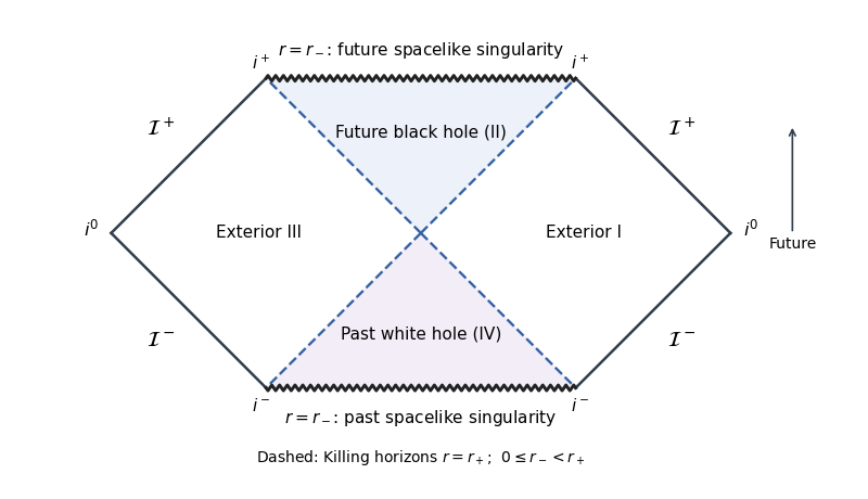
Given an asymptotically flat spacetime with a conformal completion and future null infinity ${\mathcal{I}}^{+}$, its black hole region isThe event horizon is its boundary. For the magnetically charged dilaton black hole, first assume $0\le a=r_{-}<b=r_{+}$. The physical asymptotic component has $r>a$, and the ingoing chart extends regularly across $r=b$. Its future ingoing null direction is $-{\partial }_r$. For $a<r<b$,Hence $\nabla r$ is future timelike. Every nonzero future causal tangent $X$ satisfies $X(r)=g(\nabla r,X)<0$. A future causal curve from this interior can neither cross back to $r=b$ nor reach the asymptotic end $r\to \infty$, so it cannot reach ${\mathcal{I}}^{+}$. It lies in $\mathcal{B}$.

This proof uses the future black-hole extension. The radial interval alone does not distinguish it from the past white hole interior of the maximal extension; that interior has the same interval and can send signals to infinity. Thus the statement needs this future-component qualification if the maximal spacetime is intended.

The Kretschmann scalar confirms that $r=a$ is a genuine curvature singularity: for $0<a<b$, its numerator at $r=a$ is $3a^4(a-b{)}^2$, andFor $a=0$ it instead reduces to $12b^2/r^6$. Since $V<0$ on approaching the singularity from the interior, the singularity is spacelike. At $r=b>a$ the curvature is finite.

For the maximal extension, take $U=-e^{-u/(2b)}$, $W=e^{v/(2b)}$ in the right exterior and continue analytically across the horizons. ThenThe singularity is $UW=(1-a/b)e^{a/b}>0$ and the horizons are $U=0$ and $W=0$. Rescaling the null coordinates by the square root of this positive constant before arctangent compactification produces the usual qualitative Penrose diagram of Schwarzschild spacetime: two exteriors, a future black-hole region, a past white-hole region, and future and past spacelike singularities. The dashed lines below are the horizon branches; only the future interior is the black-hole region.

If $a>b$, the physical domain remains $r>a$, but now $V>0$ throughout it. The apparent zero $r=b$ is beyond the curvature singularity and is not an accessible horizon. The singularity is timelike, and outgoing radial null rays with $\dot{r}=E>0$ escape to infinity from arbitrarily near it. ThusThe excluded equality $r_{-}=r_{+}$ is a singular limiting case, not a regular horizon. These facts describe the causal structure of the magnetic dilaton black hole.

In the regular ingoing chart, the Killing vector field is $k={\partial }_v$, with $k^2=-V$. The normal covector to $r=b=r_{+}$ is $dr$; raising its index gives $\nabla r={\partial }_v+V{\partial }_r=k$ at $r=b$. Thus $k$ is null and normal to that hypersurface, which is a Killing horizon. It is regular because $R^2(b)=b(b-a)>0$ when $a=r_{-}<b$.

The defining identity for surface gravity on a Killing horizon is ${\nabla }_a(k^2)=-2\kappa k_a$. Here $k_a=-V(dv{)}_a+(dr{)}_a$, so at the horizon this becomes $-V^{\prime }(b)(dr{)}_a=-2\kappa (dr{)}_a$. ThereforeThis uses the asymptotic normalization $k^2\to -1$. A constant rescaling of $k$ rescales the surface gravity. As a check, the horizon area is $A_H=4\pi r_{+}(r_{+}-r_{-})$ and $\kappa A_H/(4\pi )=(r_{+}-r_{-})/2=M_{\mathrm{Komar}}(r_{+})$. The formula is being applied only to the regular strict-inequality case.

For complex solutions of the Klein-Gordon equation, define the currentIts divergence isbecause $\square \beta =m^2\beta$ and $\square \overline{\alpha }=m^2\overline{\alpha }$ for real $m^2$. The Klein-Gordon inner product is the flux ${\int }_{\Sigma }{n}_a{j}^{a}d\Sigma$. Applying Stokes theorem to a slab between two Cauchy hypersurfaces gives equality of the fluxes, with the future normal on each surface and opposite boundary orientations.

For noncompact surfaces this requires the integrals to converge and no net flux through spatial infinity, for example spacelike compact support or suitable decay. Global hyperbolicity alone does not ensure convergence for arbitrary solutions. Under these conditions,Complex conjugation also givesThus it is a Hermitian form, antilinear in its first argument and linear in its second. It is indefinite on the full complex solution space; positivity will arise only on a chosen positive-frequency solution subspace.

In Minkowski spacetime with signature $(-+++)$, $p\cdot x=-{\omega }_{\mathbf{p}}t+\mathbf{p}\cdot \mathbf{x}$, where ${\omega }_{\mathbf{p}}=p^0=\sqrt{|\mathbf{p}{|}^2+m^2}>0$. Hence $i{\partial }_t{\psi }_{\mathbf{p}}={\omega }_{\mathbf{p}}{\psi }_{\mathbf{p}}$: these are positive-frequency solutions relative to the inertial time translation.

On a constant-time Cauchy hypersurface, the Klein-Gordon inner product and the spatial Fourier transform identity giveAlso $({\overline{\psi }}_{\mathbf{p}},{\overline{\psi }}_{\mathbf{q}})=-{\delta }^3(\mathbf{p}-\mathbf{q})$ and $({\psi }_{\mathbf{p}},{\overline{\psi }}_{\mathbf{q}})=0$: the latter is proportional to $({\omega }_{\mathbf{p}}-{\omega }_{\mathbf{q}}){\delta }^3(\mathbf{p}+\mathbf{q})$, which vanishes. This is the Klein-Gordon plane-wave normalization.

For completeness, spatial Fourier transformation of the field equation gives $\ddot{\hat{\Phi }}(t,\mathbf{p})+{\omega }_{\mathbf{p}}^2\hat{\Phi }(t,\mathbf{p})=0$. Its solutions have the two branches $e^{\mp i{\omega }_{\mathbf{p}}t}$. Selecting the positive-frequency branch leaves precisely the Fourier superpositions of ${\psi }_{\mathbf{p}}$. These plane waves form a generalized basis, normalized with the Dirac delta distribution, rather than individually normalizable vectors. For a normalizable packet,

The Klein-Gordon inner product satisfies $(\overline{\alpha },\overline{\beta })=-(\beta ,\alpha )$, so $({\overline{\psi }}_i,{\overline{\psi }}_j)=-{\delta }_{ij}$. Orthogonality of positive and negative modes in the field expansion therefore gives $({\psi }_i,\Phi )=a_i$ and $({\overline{\psi }}_i,\Phi )=-a_i^{†}$.

Extracting the primed coefficient in the same way, and using antilinearity in the first entry,Consequently the Bogoliubov transformation of the creation and annihilation operators isThe minus sign comes from the negative norm of the conjugate modes, and the complex conjugates come from the first argument of the Hermitian pairing.

Use the canonical commutation relation for the creation and annihilation operators and the transformation derived above. Directly,Requiring these to equal ${\delta }_{ik}$ and zero, respectively, and conjugating the equations yields the canonical identities for a bosonic Bogoliubov transformation:The commutator of the primed creation operators then vanishes by taking adjoints. These are exactly the corresponding positive-mode norm and positive-negative orthogonality conditions for the Bogoliubov transformation. They are sufficient for these algebraic commutators whenever the sums are well defined. Infinitely many modes introduce further questions of convergence and whether the two choices admit a common bosonic Fock space representation; the matrix identities alone do not settle unitary implementability.

Choose the unprimed modes as the inertial positive-frequency modes in the far past, and the primed modes as those in the far future. In the in-vacuum and out-vacuum construction, $|0_{\mathrm{in}}⟩$ is annihilated by every $a_j$. The number of late-time quanta in mode $i$ is measured by $N_i^{\prime }=a_i^{\prime }{}^{†}{a}_i^{\prime }$. Expanding using the Bogoliubov transformation, the only surviving vacuum contraction is $⟨0_{\mathrm{in}}|a_j{a}_k^{†}|0_{\mathrm{in}}⟩={\delta }_{jk}$. Thus the particle number from Bogoliubov coefficients isIf $B\ne 0$, at least one row has positive norm and late-time observers detect particles. If $B=0$, each $a_i^{\prime }$ is a linear combination of past annihilation operators and annihilates the same state, so all these occupation numbers vanish. The intervening nonstationary geometry can mix positive and negative frequencies, realizing vacuum ambiguity in a nonstationary spacetime even though the asymptotic inertial choices are unambiguous.

For infinitely many modes, the expressions are understood with suitable convergence or wave-packet regularization. The total expected number is ${\sum }_{ij}|B_{ij}{|}^2$, finite precisely when $B$ is a Hilbert-Schmidt operator in the specified orthonormal mode spaces. A divergent sum is not a finite occupation number in a common vacuum representation; it signals the extra infinite-dimensional issue rather than changing the finite-mode calculation.