Differentiation under the integral gives . Integrating the derivative of and then once more yields .
Completing the square gives , so each marginal is . Their covariance is , so they are not independent.
From part (i),The conditional-normal formula therefore givesConsequently the Gaussian conditional expectation is
Apply part (ii): .
, so .
Substitution and cancellation give .
Equating powers gives .
, so the critical points are . The Hessian matrix at is , making it the local minimum; is degenerate and not a minimum.
. The descending gradient flow trajectory from stays in its bounded contour basin and tends to the only critical point there, .
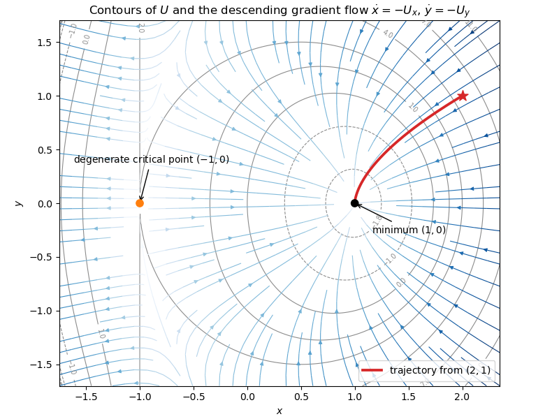
Contours and descending gradient flow for the 2026 Paper IA 2 potential
. Contour lines of U equal x cubed minus 3x plus open parenthesis x plus 1 close parenthesis y squared are overlaid with the descending gradient field. The highlighted trajectory starts at open parenthesis 2 comma 1 close parenthesis and tends to the local minimum at open parenthesis 1 comma 0 close parenthesis; the other marked critical point is degenerate.The roots are . They give oscillatory decay for , two exponential decays for , and at equality. All tend to zero.
Put , , and . A solution satisfying both endpoint conditions iswhere . The derivative jumps by at , as required.
Substitution gives . Multiply by and integrate over ; decay kills the first and last integrals, leaving . Thus a nonconstant profile requires and approaches a fixed position.
During warming, and . During cooling, with , and .
Chebyshev inequality gives .
Only triangle pairs sharing an edge have nonzero covariance, soAfter division by this is for , ; use part (iii).
The word has no proper self-overlap, so its mean waiting time is the reciprocal of its probability: . This also follows from two first-step equations.
The standard run recursion gives .
For , . It is the sum of independent geometric variables, so the central limit theorem applies with mean and standard deviation . Take
and .
and .
At time the visited vertices form a contiguous arc and the walk is at an endpoint. Exiting an interval of visited vertices, starting one step from an absorbing endpoint, has mean . Therefore and .
For each , cut the cycle at . The event that is last is the event that the lifted walk covers the other residues before crossing that cut. Gambler’s ruin (or cyclic symmetry of the two expanding endpoints) gives .
Conditioning on generation and using independence gives .
Differentiating at gives , hence .
The extinction probability is the smallest fixed point of the convex generating function in . Since and make strict convexity relevant, the only fixed point is .
Articles by others on the same topic
There are currently no matching articles.