For a real random variable with finite variance , expected value , and a threshold , Chebyshev's inequality givesOne can also cap this upper bound at one, since a probability cannot exceed one. If , taking gives . For example, at least of the probability lies strictly within two standard deviations of the mean. This statement needs only the finite variance assumption. If the variance is zero, almost surely and every positive deviation threshold has zero tail probability.
Consider a random variable uniformly distributed on . Its expected value is zero and its variance is . At the actual tail probability is , while Chebyshev's inequality gives . At the actual tail probability is zero, while the bound is . A valid bound need not describe the exact shape or bounded support of a particular probability distribution.
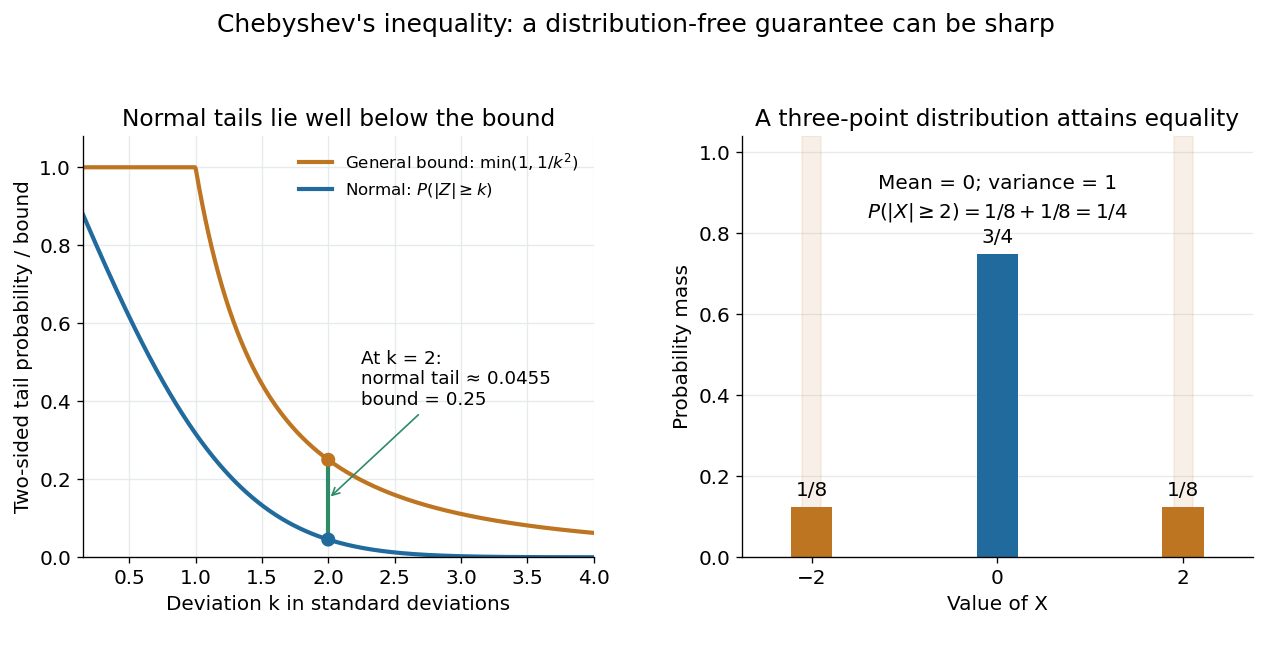
For the standard normal distribution, the actual tail probabilities beyond two and three standard deviations are approximately and , whereas the general bounds are and . More knowledge of the probability distribution can therefore improve the estimate. The comparison does not diminish the guarantee: the three-point example in equality in Chebyshev's inequality attains it exactly.
The proof is a one-line use of Markov's inequality on the nonnegative random variable . The event equals , and . This explains why the denominator is squared and why a finite variance supplies the necessary information. [ref]
https://ocw.mit.edu/courses/18-175-theory-of-probability-spring-2014/887e96172e82a615dac16fb26702d88b_MIT18_175S14_Lecture8.pdf. Scott Sheffield, MIT 18.175, lecture 8: Markov and Chebyshev bounds
.One important use is control of a sample mean. For independent and identically distributed random variables with finite variance , the variance of a sample mean is . HenceFor every fixed tolerance, the bound tends to zero as the sample size grows, proving the finite-variance case of the weak law of large numbers. For and , makes the bound . This is a sufficient bound under the stated assumptions, rather than an optimal required sample size.
An early historical source is Pafnuty Chebyshev's 1867 paper “Des valeurs moyennes”, published in French translation by N. de Khanikof. Its opening theorem bounds deviations of sums using their expected values and second moments, linking averages with control of exceptional outcomes. [ref]
https://www.numdam.org/item/JMPA_1867_2_12__177_0.pdf. Chebyshev, Journal de mathématiques pures et appliquées, 2nd series 12, 177–184 (1867)
.An unbiased coefficient estimator with known variance gives a conservative level- test of a zero coefficient by rejecting when its absolute value is at least . Chebyshev's inequality bounds the null rejection probability by . This test needs the variance assumptions but no Gaussian error distribution; a normal-reference test requires additional distributional justification.
For , assign probability to each of and , and the remaining probability to . This probability distribution has expected value , variance , and tail probability . Thus Chebyshev's inequality is sharp when only these two moments are supplied. For example, , , gives masses , , . Replacing with would exclude the two extreme points in this example.
Cantelli's inequality uses a mean and variance to control deviations in one specified direction. For a real random variable with expected value , finite variance , and ,Applying the same statement to gives the lower tail probability bound . No independence or particular probability distribution is required. If , the random variable equals almost surely and both positive-threshold tail probabilities are zero.
For variance one and a threshold two above the mean, the upper-tail probability is at most . Applying the two-sided Chebyshev's inequality to contain that upper event would give the weaker bound . For the standard normal distribution, the actual upper tail probability at two is about , much smaller than either bound. Yet the two-point probability distribution in equality in Cantelli's inequality attains , showing why the smaller Gaussian value cannot be promised from these two moments alone.
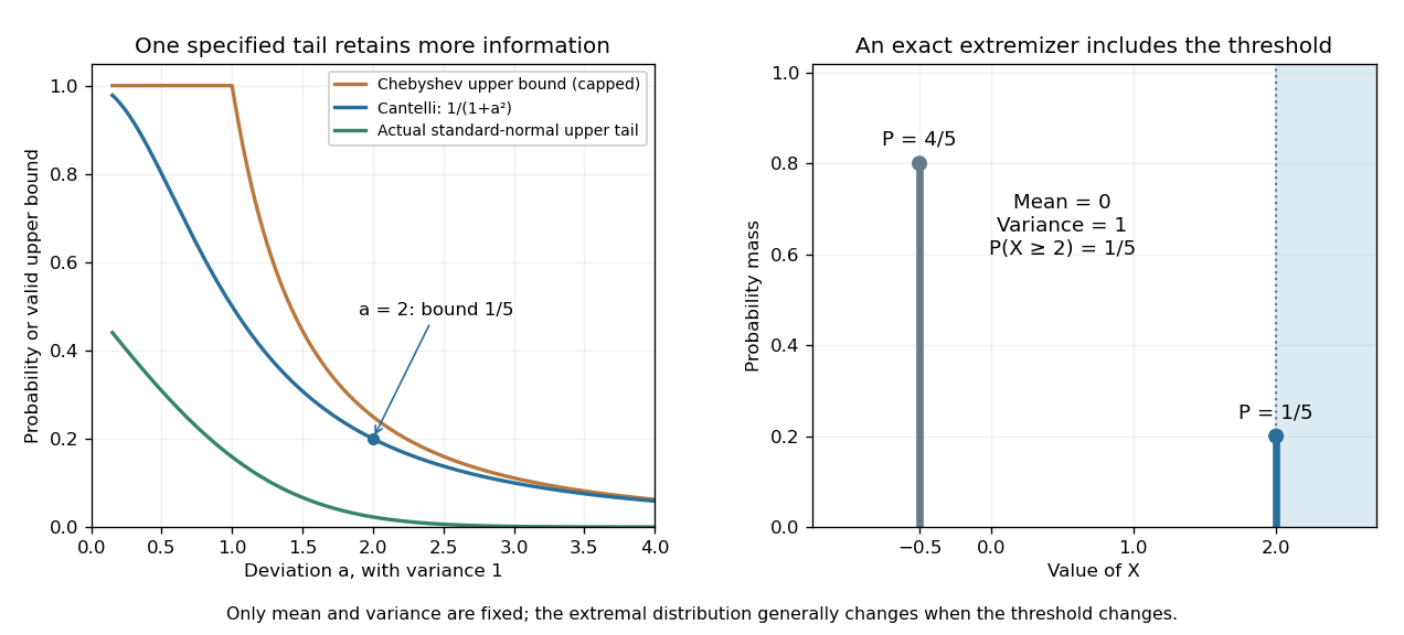
Cantelli's inequality sharpens a variance-only upper-tail bound and is exact for a two-point probability distribution
. Left: actual upper tail probabilities for the standard normal distribution are compared with Cantelli's inequality and the capped two-sided Chebyshev's inequality used as an upper-tail bound. Right: masses at and at two have mean zero and variance one. The upper mass is included by the non-strict threshold . These are specified mathematical models, not observations. Details.A short explanation is to centre and choose a nonnegative shift . On , the square is at least , so Markov's inequality givesThe best shift is , giving the displayed bound. Choosing the shift before squaring exploits the direction of the deviation; squaring the unshifted random variable treats both directions together. This shifted-square proof is also the strategy requested in the University of Utah's 2005 qualifying problem on Cantelli's inequality. [ref]
https://quals.math.utah.edu/topics/borel-cantelli-lemmas/. University of Utah Mathematics, 2005 question 4: shifted-square Cantelli bound
.The one-sided improvement should be used for a one-sided question. Adding upper and lower bounds by the union bound gives for . When , that is at least the Chebyshev's inequality bound ; when , both two-sided expressions exceed one and must be capped. The separate one-sided bounds generally cannot be attained simultaneously by the same probability distribution.
For and , place probabilitiesTheir weighted deviations cancel, giving expected value ; their weighted squared deviations give variance . Only the upper point belongs to , so its tail probability attains Cantelli's inequality. With , , , the locations are two and , with masses and . The optimized shift makes the lower point zero before squaring, explaining equality in the Markov's inequality step.
The threshold convention matters: this example has . For a strict threshold, placing the upper point at instead gives probabilities approaching the same bound as , with the prescribed mean and variance retained. Extra restrictions on the support of a probability distribution can change which extremal models are allowed.


