Past exam of the MPhil in micro- and nanotechnology enterprise course of the University of Cambridge / 2019 / Paper 1 / Section A(i)

The repeated, similarly oriented rounded triangular outlines in panel (a) are characteristic of AFM tip convolution: a narrow raised object can image the shape of a blunt or contaminated AFM probe, rather than reveal its own lateral shape. A finite tip radius broadens lateral dimensions. Replace or clean the AFM probe, check it on an independently characterized sharp-feature standard, and repeat at low load; agreement after a tip change is stronger evidence than a visually pleasing image. Image processing cannot uniquely recover unmeasured sidewalls or prove that every particle with a similar outline is an artefact.

Panel (b) contains horizontal streaks associated with steep features. The natural instrumental diagnosis is AFM feedback artefact: the height controller does not track a rapid change faithfully, or rings after it. Reduce the scan speed and adjust proportional/integral gains below the oscillation threshold. Compare trace and retrace and rotate the fast-scan direction: a streak following the scan rather than the specimen is instrumental. Loose contamination can also produce scan-line streaks, so clean or change the AFM probe if tuning does not remove them. Tip-shape broadening in (a), and scan-direction tracking/streaking in (b), are the principal diagnoses; the images alone do not uniquely establish every underlying cause.

piezoelectric scanner creep is the continued slow displacement after a step in scanner drive, even when the commanded voltage has stopped changing. The scanner's strain continues to relax, and the motion can resemble a slowly decaying, approximately logarithmic drift. After changing scan size, position or offset, early lines can therefore have stretched or compressed coordinates. Allow settling, avoid large abrupt moves, use a position-sensor closed-loop control system, and compare repeated images. This time-dependent response differs from the direction-dependent piezoelectric hysteresis and from ordinary thermal drift.

A steady-current image is not supported by the electrical connection drawn. tunnelling atomic force microscopy requires a conducting AFM probe, an applied bias voltage and a continuous return path from the contacted region to the current amplifier. graphene is conducting, but a flake on insulating glass is not electrically grounded merely because the other side or edge of the glass is earthed. Charging transients or displacement current are not its steady conductivity. Add a metal contact actually touching the graphene before using its current contrast; ordinary force-based surface topography can still be recorded without that contact. The manufacturer's nanostructure measurements explicitly distinguish objects connected to conducting pads from unconnected particles on the same insulating substrate.^[ref]

quantitative nanomechanical mapping can image the flake without an electrical return path. Repeated AFM force curves provide surface topography, adhesion and deformation or effective elastic modulus channels. The step and differences in tip–surface interaction can distinguish graphene from glass. For an atomically thin supported sheet the contact response is strongly substrate dependent, so fitting a three-dimensional half-space contact model does not directly measure the intrinsic in-plane Young's modulus of free graphene. Calibrate the cantilever spring constant, deflection sensitivity and tip radius, use small loads, and compare bare substrate. The manufacturer's description specifies the force-curve origin of the mechanical channels.^[ref]

friction force microscopy is suitable. Contact scanning twists the AFM cantilever; the lateral photodetector difference measures friction and can distinguish the supported graphene and glass even if their heights are close. Acquire both trace and retrace and use half their lateral-signal difference to suppress slope-induced cross-talk. Keep the normal load low enough to avoid dragging or damaging the flake, control humidity and contamination, and calibrate torsional sensitivity if a quantitative coefficient of friction is required. An electrical connection is unnecessary.

Conventional semiconductor scanning capacitance microscopy is not a reliable dopant-contrast image of this specimen as drawn. Its usual $dC/dV$ signal relies on a tip–insulator–semiconductor capacitance whose depletion region changes under AC bias. An isolated conducting graphene sheet on thick insulating glass provides neither that conventional depletion geometry nor a controlled charge reservoir; simply earthing glass does not supply one. Capacitive or electrostatic contrast may be detectable with a suitably designed back electrode, a contacted flake and an appropriate capacitance-sensitive instrument, but that is an additional electrical device specification. Force-based surface topography remains possible independently of the specialized capacitance channel.

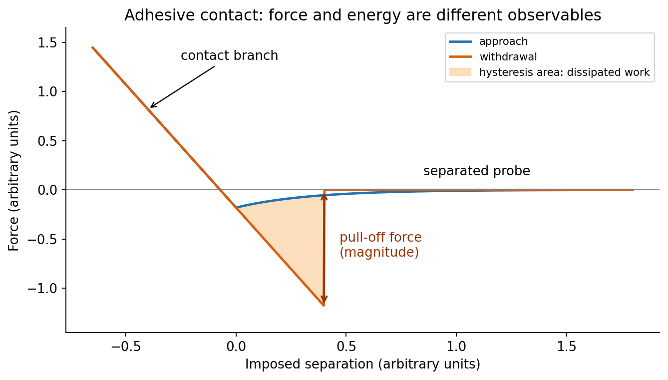
At position (1), the AFM probe is far from the surface, with approximately zero force. At (2), attractive interactions bend the AFM cantilever toward the surface; when the attractive force gradient exceeds the cantilever spring constant, the equilibrium becomes unstable and jump-to-contact occurs. Position (3) is on the mechanical-contact branch: changes in imposed height largely bend the AFM cantilever and, for a compliant specimen, indent the sample. This branch can include compressive contact and adhesive contact under tension; contact does not itself imply a positive force at every point. At (4), during withdrawal the tip remains attached and pulls the AFM cantilever downward until the pull-off force is reached and it detaches. Approach and retraction follow different paths because adhesion creates a hysteretic contact. The numbered points identify stages on the source curve, not four extra question parts.

In quantitative nanomechanical mapping, the operational adhesion is the magnitude of the most attractive force immediately before detachment on a calibrated retraction curve:Here $k_c$ is the cantilever spring constant and ${\delta }_c$ its deflection after baseline subtraction. The area between approach and retraction relates to dissipated work, whereas the minimum force is a force, not an energy. Chemical attraction, Van der Waals forces and ambient-water capillary bridges can all contribute. Match loading rate and peak load, calibrate deflection sensitivity and $k_c$, compare clean reference surfaces, and control humidity; otherwise different maps may reflect different tips or capillary conditions rather than different specimens.

Three suitable approaches give complementary contrast. tapping-mode atomic force microscopy supplies surface topography and an oscillation-phase image. It reduces lateral drag and is often effective for soft block copolymer domains. Its phase contrast depends on elastic response, adhesion, dissipation and operating setpoint together: a bright phase domain is not automatically the stiffer polymer. Check contrast as amplitude and setpoint change and use a known reference.

quantitative nanomechanical mapping fits the repulsive portions of many AFM force curves and separately maps effective elastic modulus, adhesion and deformation. It directly addresses the stiffness difference and limits maximum force. Its quantitative result depends on tip radius, force calibration, contact model, loading rate and film thickness; domains narrower than the contact footprint are mixed and the substrate can dominate a thin film. Use small indentation, substrate controls and a suitable viscoelastic interpretation.

friction force microscopy can reveal domains with different frictional and adhesive response, using torsional deflection during contact scans. It is simple and sensitive to surface chemistry, but continuous shear may deform or displace soft domains, and slope/topography can contaminate the lateral signal. Acquire trace–retrace pairs at several low normal loads and check reproducibility. Use a mechanical-modulus map to test the stiffness assignment; phase or friction contrast alone does not uniquely identify stiffness or chemical composition.