An orthogonal projector sends to the foot of its perpendicular onto the image of a linear map . The residual is orthogonal to the entire range, not just to the single vector . Indeed, for any range vector ,In particular . The orthogonal projection diagram illustrates the resulting right triangle.
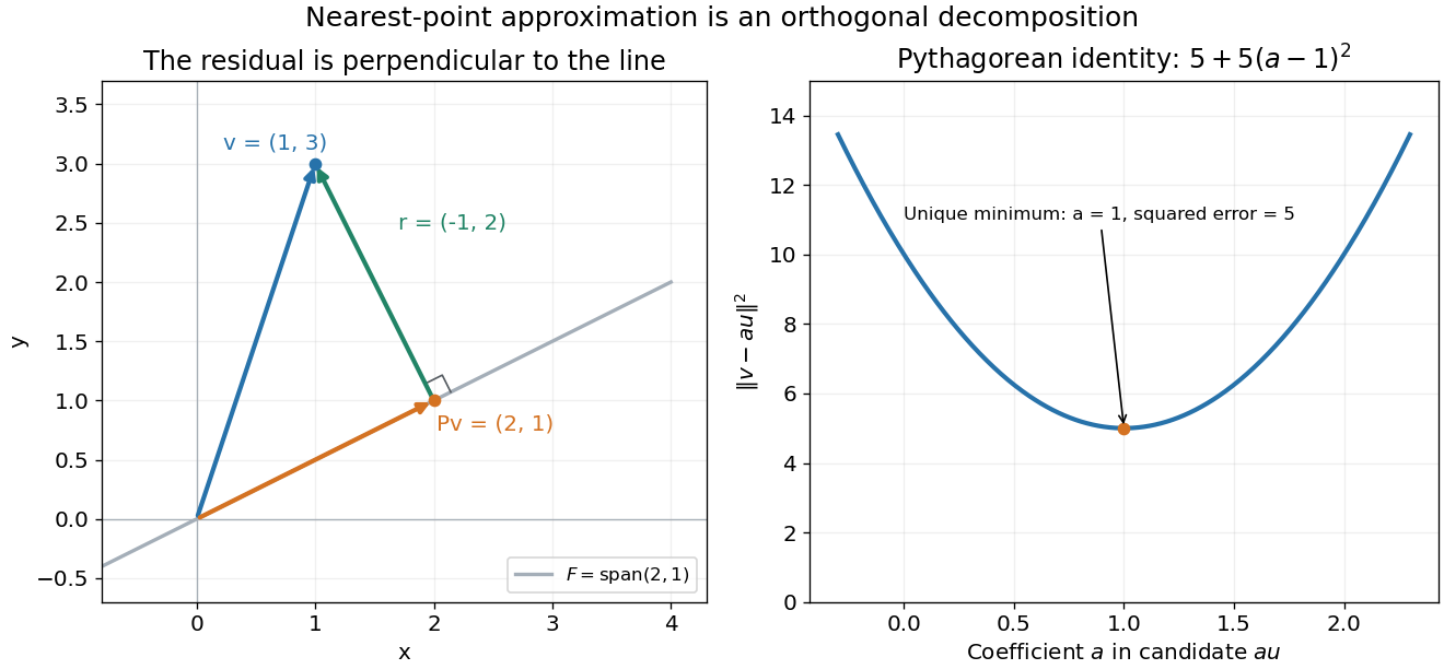
An orthogonal projector maps a vector to its perpendicular foot on the range; the residual is orthogonal to that range
. Details. 
The vector Euclidean norm is , the ordinary length from the origin. The induced matrix norm isGeometrically this is the largest stretch of a unit vector. A linear map sends the unit sphere to an ellipsoid, possibly degenerate; its largest semiaxis has length . Equivalently the matrix 2-norm is the largest singular value.
The perpendicular decomposition in part (a) gives, by the Pythagorean theorem,Thus an orthogonal projection cannot lengthen a vector and . Algebraically the cross term vanishes because , giving the same identity directly from the hypotheses. If , take a nonzero in its range; then and . For the norm is zero.
The nullspace is the vector subspace . A full real singular value decomposition iswhere are orthogonal matrices and for , with for . We may order . The columns of form an orthonormal basis of the input space , and the columns of form one of the output space . The positive singular values number exactly the matrix rank.
Let be the matrix rank, and partition the right singular vectors as , with consisting of the columns associated with zero singular values. From , these columns form an orthonormal basis of the nullspace. Therefore its orthogonal projector isIt acts on the input space . Symmetry and idempotence follow from . At full column rank it is zero, and at rank zero it is the identity.
At elimination column , let be the size of the remaining trailing block. Computing its multipliers costs divisions; updating all entries costs floating-point operations, one multiplication and one subtraction per entry. Thus the dominant count isUpdating the right side and back substitution add only floating-point operations. Pivot searches involve comparisons and row exchanges, without changing the leading arithmetic count. Hence Gaussian elimination with pivoting has the requested asymptotic cost.
An orthogonal similarity transformation is with . An upper Hessenberg matrix has whenever ; its first subdiagonal may be nonzero.
At step , choose a Householder reflector whose trailing block sends the current column segment in rows to a multiple of its first coordinate. The left multiplication zeros positions . Apply the matching right multiplication to retain similarity: . Since acts only on rows and columns , earlier Hessenberg zeros are preserved. Finally gives .
Each reflector is applied through a rank-one update, costing rather than a full matrix multiplication. Across steps, the Hessenberg reduction costs .
Solving the unrelated shifted systems by separate Gaussian elimination costs floating-point operations.
Instead compute once in work. For each shift, solveThe shift changes only the diagonal, so remains an upper Hessenberg matrix. In each elimination column only the entry immediately below the pivot needs removal. With partial pivoting the only possible nonzero candidate rows are the current row and the next, and each update touches entries. Factorization therefore costs per shift; the triangular solve and both orthogonal-vector transformations also cost each.
Thus shifted solves plus the initial Hessenberg reduction cost in total. Pivoting is still needed in general: nonsingularity excludes a singular system but does not by itself guarantee that every unpivoted elimination pivot is nonzero.
The off-diagonal Toeplitz matrix is symmetric and has row and column absolute sums bounded byFor an elementary Euclidean bound, apply the weighted Cauchy-Schwarz inequality in each row:Sum over and use both absolute-sum bounds to get . ThereforeThe entry is unused because the diagonal of is fixed to one; including it only weakens the bound. This is the row-column bound for the matrix 2-norm.
A real symmetric matrix is positive-definite when for every nonzero real vector . The preceding matrix 2-norm bound givesThus is a symmetric positive-definite matrix, independently of the detailed positions of the nonzero entries of .
An eigenvalue of is a scalar for which has a nonzero eigenvector. Allowing initially , symmetry of the real matrix gives , so is real. Since ,This proves reality without presuming it when choosing the eigenvector. Once is real, the real or imaginary part of supplies a nonzero real eigenvector.
For a unit eigenvector of , . The matrix 2-norm bound from part (a) gives . Hence every eigenvalue lies inIn particular the condition number in the Euclidean operator norm satisfies .
The energy norm associated with this symmetric positive-definite matrix isIt is the norm induced by the inner product . The conjugate gradient method minimizes this error norm over its successive affine Krylov subspaces.
The standard conjugate gradient convergence bound isHere , so the factor in parentheses is at most . Since , 25 iterations suffice to reduce the energy-norm error by a factor exceeding .
There are at most nonzero entries of , and each contributes to at most two off-diagonals. Thus has at most nonzero entries. Initialize a matrix-vector product with the diagonal contribution , which costs no arithmetic because the diagonal is one. Each off-diagonal term needs one multiplication and one addition, giving at most floating-point operations per product.
A standard conjugate gradient step adds two inner products, three vector updates and two scalar divisions, at most further operations. Starting from makes and avoids an initial matrix-vector product; its squared norm needs operations. The total for 25 steps is at mostThis supplies an explicit meaning of the paper's large- qualification. The quoted conjugate gradient convergence bound is the usual exact-arithmetic result.
Articles by others on the same topic
There are currently no matching articles.